Assuming that all routes connecting any two processors are composed of links .... across a route of the star-of-stars as shown in Figure 3, where T_LOP(i) is the ...
Using Parallelism and Pipeline for the Optimisation of Join Queries Maria Spiliopoulou, Michalis Hatzopoulos, Costas Vassilakis1 Department of Informatics, University of Athens Panepistmiopolis, TYPA Bldgs, Ilisia, GR 157 71 Abstract: In this study we present a technique for the parallel optimisation of join queries, that uses the offered coarse-grain parallelism of the underlying architecture in order to reduce the CPU-bound optimisation overhead. The optimisation technique performs an almost exhaustive search of the solution space for small join queries and gradually, as the number of joins increases, it diverges towards iterative improvement. This technique has been developed on a low-parallelism transputer-based architecture, where its behaviour is studied for the optimisation of queries with many tenths of joins.
1 Introduction One of the problems recently addressed in database research is the optimisation of large join queries. Conventional optimisation models are based on exhaustive techniques, the overhead of which increases exponentially with the query size [12]. Therefore, researchers focus on techniques based on iterative improvement, like Swami and Gupta [12, 13], or simulated annealing, like Ioannidis, Wong and Kang [2, 3], aiming at a polynomially increasing optimisation overhead. Query optimisation techniques arc CPU-intensive applications; so they may benefit from parallelism. Both exhaustive techniques, which construct all query execution plans to find the optimal one, and non-exhaustive techniques of iterative nature, like iterative improvement and simulated annealing, are clearly parallelisable. In this study, we propose a query optimisation model, which uses parallelism not only for query execution but also for query optimisation. We present a parallel optimisation technique which is almost exhaustive for small join queries and diverges gradually from exhaustive techniques for larger queries towards iterative improvement. The overhead of this technique is less than the overhead of an exhaustive strategy and is further reduced proportionally to the utilised processors. The paper is structured as follows: In the next section, we make a brief overview of query optimisation techniques. In section 3, we focus on parallel environments and outline the query processing model, for which the optimisation technique is designed. In section 4, we analyse the parallel optimisation technique. Section 5 presents the first results of an experimental implementation of the model on a transputer machine. The final section concludes the paper and presents some future extensions of the model.
1
Part of this work is performed within the project 4061 Parallel Computing Action (PCA), partially funded by the CEC.
2 Optimisation Techniques for Join Queries Query optimisation aims at the selection of an optimal access plan out of all plans that can be constructed by placing the query operators in all possible orderings and assigning to them any of the execution algorithms available in the literature. Adopting the terminology of combinatorial optimisation problems, each query access plan can be observed as a state in the space containing all solutions to the problem. The optimal state is obviously a state of the solution space that has lowermost cost. In most query models, query optimisation is reduced to the optimisation of join operators, which in turn is reduced to finding the best join order and to assigning the most appropriate algorithm to each of the joins, as analysed by Ioannidis and Kang [4]. In this study, we also focus on the optimisation of join queries, although the impact of other operators on the access plans and, especially, on the optimisation process itself also deserves a thorough study, as mentioned elsewhere [9]. As pointed by Ioannidis and Kang [4], a state in the solution space of the join query optimisation problem corresponds to the access plan for a "join processing tree" [4]. The join processing tree is a special case of a query tree, the nodes of which are query operators, while the vertices represent the flow of information from the leaves obtaining the relations from secondary storage towards the root producing the final output. The join processing tree is thus a query tree comprised solely of JOIN-nodes. The exhaustive searching of the solution space in order to select the state with the minimum cost has a rapidly increasing overhead, since the number of states grows exponentially to the number of operators in the query. Thus, the optimisation overhead reaches unacceptably high values, especially for large join queries, as mentioned by Swami and Gupta [12]. In the model of Selinger et al [7] the optimisation overhead is reduced by the use of heuristics, which exclude a number of states from the solution space as potentially suboptimal. However, the combinatorial nature of the problem is not overcome: as recent research focuses on the optimisation of large join queries, the usage of optimisation techniques of exhaustive nature becomes inappropriate. In order to optimise large join queries, researchers focus on "randomised algorithms", which are used in an iterative fashion, as described by Ioannidis and Kang [3]. The iterative techniques employed are based on iterative improvement, as in the models of Swami and Gupta [12] and Swami [13], on simulated annealing, as in the model of Ioannidis and Wong [2], and on combinations of the two, as in the model of Ioannidis and Kang [3, 4]. The models of Swami and Gupta [12, 13] use a special type of join processing tree, the Outer Linear Join Tree (OLJT). The main characteristic of the OLJT is that for each JOIN-node it holds that the inner operand relation is always a base one. By using only the hash algorithm for all joins, the optimisation problem is further reduced to that of finding the optimal join ordering. To resolve this problem, the iterative improvement technique combined with augmentation heuristics is suggested as the most efficient approach [13]. The model of Ioannidis and Wong [2] uses simulated annealing, while the model of Ioannidis and Kang [3, 4] combines simulated annealing with iterative improvement for deep and bushy join processing trees, which are more general than the left-deep OLJTs. The study shows the superiority of the composite technique, called 2-phase optimisation, for all solution spaces but those where local minima are scattered at all costs [4].
The aforementioned approaches leave an intermediate area of solution spaces for deep and bushy trees, where local minima are scattered at all costs. Moreover, in both optimisation techniques both the exhaustive ones and those based on randomised algorithms, the fact is overseen that the optimisation overhead can be reduced in much the same way as the execution cost of the queries, namely by using the available processing power of the parallel machines, on which the database models operate.
3 The Environment of the Parallel Optimisation Technique The primary objective of most query optimisers is the minimisation of query execution time. Since database research has focused on the optimisation of large join queries, the minimisation of optimisation overhead becomes an additional objective for modern query processing models. Our optimisation model utilises parallelism to minimise both the (usually I/O-bound) execution time and the CPU-bound optimisation overhead. The model is designed for coarse-grain parallelism architectures comprised by a small number (a few tenths) of processors with private memories, point-to-point interprocessor communication and shared peripherals; however, the proposed technique can also be used on machines with private peripherals per processor. These architectures conform to the requirements of recent database machines, as identified in the overview of De Witt and Gray [1]. The model transforms the initial query into the query tree representation we proposed in [11]. Since in this study we focus on the optimisation of join queries, we only consider join processing trees, hereafter also denoted as JTs; however, the same technique is applicable when all query operators are considered, as in the model we propose in [9]. The JTs handled by our model are both deep and bushy, like the JTs addressed in the model of Ioannidis and Kang [4]. This tree structure has two advantages: (i) It reduces the optimisation problem to that of finding the optimal join order and the most appropriate algorithms for the nodes [4], as already noted, and (ii) it is very suitable for low parallelism architectures, since it can be directly mapped one-to-one into the query execution graph on the parallel machine; tree nodes are mapped into execution tasks, while tree vertices are implemented as pipes on the execution graph. The optimal join tree for a query is a join tree with smallest cost, constructed by repeated tree reorganisation and algorithms' selection. The optimiser uses a library of uniprocessor join algorithms, since the model runs on a low parallelism environment, where each tree node is executed by a single processor. The following join algorithms are available for all join operators, including the anti-join operator introduced by Kim [5]: • the classic hash method for joins and outerjoins bearing the equality operator, as well as for anti-joins • the nested loops method for joins on relations, one of which fits in a processor's main memory • the merge method for joins on relations, all of which are sorted on the join attribute The execution algorithm assigned to a JOIN-node is not randomly selected, as in the model of Ioannidis and Kang [4], because the behaviour of the three aforementioned algorithms is well studied, as in the work of Kim [5], Shapiro [8] and Mikkilineni and Su [6], so that criteria for their usage can be extracted:
1. The classic hash method shows best behaviour when the relation on which the hash table is constructed fits in a processor's memory, as proven by Shapiro [8]. The method can still be used even if only the hash table fits in memory, since this algorithm is proven to be superior to the other two methods in most cases, as noted by Swami and Gupta [12]. 2. The nested loops algorithm performs optimally when the relation selected as inner one fits in memory. This algorithm has the further advantage of being applicable to all kinds of joins, irrespective of their comparison operator. 3. The merge algorithm requires both input relations to be sorted on the join attribute. Whenever this can be ensured, this algorithm is the more appropriate one. Otherwise, it is inferior to the hash method. Its superiority or inferiority towards the nested loops method depends on whether the cost of sorting the input relations exceeds the cost of swapping one of them in and out of secondary storage, as described by Kim [5]. The algorithm's selection for each node is performed according to these criteria.
4 Tree Reorganisation in a Parallel Environment In this section, we first analyse the sequential reorganisation technique and then describe the usage of parallelism in its implementation. 4.1 States and Moves for Tree Reorganisation Adopting the terminology used by Swami and Gupta [12], and by Ioannidis and Kang [4] for non-exhaustive optimisation techniques, we use the following terms: The initial state of the query optimisation technique is the JT input to the optimiser. On this tree a set of moves is applied, denoted as "set of transformation rules" in [4]. A move is called legal, if it produces a state having lower execution cost than the state it was applied on. The states produced by applying a move to a state S define the neighbourhood of S and are called neighbours of S [4]. The technique of iterative improvement starts by applying random moves on each of the start states, in order to produce a local minimum [12]. The start state is a state constructed by random placement of operators or by using augmentation heuristics, as in the model of Swami [13]. The local minimum with the lowermost cost among the computed ones is declared as the global minimum [12]. In the proposed technique we use: •
the swap(Join1 , Join2) move and
•
the reroot(State,Join0) operation for the construction of start states
The swap() move, shifts the positions of the nodes Join1 and Join2, which must be adjacent. swap() directly affects the position of all successors of the two nodes, but its impact on the execution plan spreads across the whole tree: the procedure assigning algorithms to the nodes is invoked for the new tree, thus constructing a new state execution plan. The arguments to the reroot() operation are the current state, which corresponds to a JT rooted at a JOIN-node JoinX, and a node Join0 other than JoinX. This operation creates a new JT rooted at node Join0 and having all other nodes of the JT placed below Join0. The
placement of nodes takes place using the mechanism, we proposed in the pre-optimisation model of [11], which ensures that tree pipeline is not corrupted, i.e. that adjacent nodes are applied at least on one common relation. The result is an equivalent JT of different structure. As in the case of swap(), algorithms are assigned to all nodes of this tree anew, thus producing a new state. In order to compute a state's cost, we developed a set of cost formulae, which are estimating the I/O and communication cost required by each strategy for execution in a parallel environment. The formulae are skipped here due to lack of space; they are proposed in ([10]). They are based on the following guidelines: (a) tree nodes are executed as tasks in parallel and pipelined fashion, (b) tasks exchange data asynchronously, (c) all algorithms filter out attributes not used in ancestor nodes and (d) projections perform sorting and (occasionally) duplicates' removal.
4.2 Description of the Tree Reorganisation Technique The tree reorganisation technique creates N neighbours of the initial state Sinit using the reroot() operation. Those neighbours are used as start states; on each start state S, a procedure SCAN() is applied, which repeatedly calls swap() to search the neighbourhood of S in an almost exhaustive way. The SCAN() procedure operates on a start state S, applying the swap() move in a loop fashion as follows: •
The start state is marked as the current state. The first JOIN-node (in a postorder traversal) in the current state is marked as current node.
•
The current node is repeatedly swapped with its ancestors, until the root of the JT is reached, maintaining the legal swaps performed in this process. The least expensive state produced by a legal swap replaces the current state; the SCAN() restarts at the first JOIN-node of the new current state. If none of the swaps is legal, the procedure marks the next JOIN-node in the postorder traversal as the current node and restarts. The procedure ends when there are no more JOINnodes to visit.
This procedure is further enhanced by ignoring improvements less than a certain percentage over the cost of the current state, so that the overhead of restarting the SCAN() in order to obtain a minor improvement is avoided. Experimentation showed that the value of 0.99 can be used as a cost improvement threshold without affecting the optimality of the solution. The swap() move is applied exhaustively on the nodes of the JT corresponding to a start state. This ensures that the neighbourhood of the start state, as determined by the swap() move, is scanned thoroughly for execution plans. Legal swaps are used to select the one with the lowest cost, and illegal ones are ignored, so that the execution plan produced for a start state is a "local optimal plan". It is local because it is optimal within the specific neighbourhood. This plan roughly corresponds to a local minimum produced by a method like iterative improvement. The swap() is restricted to the neighbourhood of a start state, which forms a small part of the search space. Therefore, it is combined with the reroot() move. reroot() defines a neighbourhood of N very different states: this neighbourhood could be classified as "sparse". For each state in this sparse neighbourhood, the swap() move produces states relatively close to each other (having differences on some locations of the corresponding
trees and on the selected algorithms): those states build a neighbourhood that can be classified as "dense". Those dense neighbourhoods are exhaustively scanned. For small trees, this technique is exhaustive, since the sparse neighbourhood defined by reroot() combined with the dense neighbourhoods defined by swap() for the start states, do cover the whole search space. Then, the behaviour of the proposed technique is close to that of an exhaustive technique. For larger trees, the technique departs gradually from the exhaustive approach, since the union of the sparse neighbourhood and the dense ones leaves areas of the search space unexplored. Then the behaviour of the proposed technique comes closer to the behaviour of iterative improvement.
4.3 Usage of Parallelism in the Tree Reorganisation Technique The technique described in the previous section is clearly parallelisable. The start states produced by reroot() can be processed independently by the SCAN() procedure applying the swap() moves. Moreover, since the arguments of reroot() are the single initial state and one JOIN-node, the construction of the different start states can also be performed in parallel. Therefore, we organise the optimisation scheme as follows: Phase 1. One master process, which acts as "coordinator", obtains the JT corresponding to the initial state. This JT is normally the output of a previously invoked query processing module, like the parser/pre-optimiser we proposed in [11]. The initial state is then produced by assigning execution algorithms to the tree's nodes. Phase 2. The coordinator activates n processes, where n is the number of JOIN-nodes in the join tree, and forwards to each of those processes the initial state, its cost and one node N, which will be used as argument to reroot(). The coordinator assures that each of the n processes receives a different node N, and that one of them will maintain the initial state as is, since the initial state is also a start state. Phase 3. Each of the n processes invokes reroot() ) and obtains a start state, by assigning algorithms to the nodes of the produced JT. Thereafter, SCAN() is activated, which computes a "local optimal plan" LOP for the start state. The cost of this LOP, denoted as T_LOP, is returned to the coordinator. Phase 4. The coordinator gathers all T_LOPs of the parallely computed local optimal plans, selects the minimum among them and then obtains the state corresponding to that T_LOP from the process that has computed it. This state is declared as the optimal execution plan for the query. The coordinator process can be optionally split in two processes, one "initialiser", which performs the tasks of Phase 1 and activates n-1 processes at the beginning of Phase 2, and one "selector", which gathers the cost estimations at the end of Phase 3 and obtains the optimal plan in Phase 4. This approach is more suitable for parallel environments where bidirectional communication among processes is not very easy to establish or is too expensive to maintain. In the following, we observe the coordinator as one logical process. The aforementioned parallel model requires the activation of n+1 processes. Since the coordinator process is idling during Phase 3, which is the potentially longer one, and since one of the n processes can avoid rerooting, because it operates on the initial state, it is more convenient to have the coordinator invoke n-1 processes and participate in Phase 3 itself, using the initial state as its start state. Thus, a total of n processes is required.
4.4 Overhead of Parallel Optimisation The parallelisation of the optimisation technique dramatically decreases the optimisation overhead to the cost of scanning the dense neighbourhood which produces the most slowly constructed LOP. Although the dense neighbourhoods can be very dissimilar and the cost of scanning each one may vary, the total optimisation cost is drastically reduced. However, the parallelisation of the optimisation technique adds an overhead that does not appear in the sequential version: the transfer of the initial state towards the n-1 processes during Phase 2, the transfer of the T_LOPs towards the coordinator during Phase 3 and the final transfer of the optimal plan towards the coordinator in Phase 4 add communication overhead. Moreover, the assignment of algorithms to the tree nodes for the construction of a state, as well as the computation of a state's cost, require metainformation on the relations, which is traditionally maintained in the data dictionary. The overhead of n processes accessing the disc in the parallel version versus a single process retrieving the dictionary in the sequential version is considerable. In order to reduce the additional overheads, the algorithm of the parallel technique is further enhanced. I/O Overhead. The meta-information of the data dictionary which is required by the optimisation technique is normally small enough to fit in main memory. Since the optimisation technique is a CPU-intensive application the available memory of a processor can be reduced to have the (necessary part of the) dictionary reside in memory, without affecting the performance of the technique. Thus, the I/O overhead is reduced to the initial loading of the dictionary file. The I/O overhead for loading the data dictionary to the n processes is reduced by having the data dictionary read from disc once by the coordinator and be subsequently broadcasted to the n-1 processes. Thus, the I/O overhead of the parallel technique becomes equal to that of the sequential version. Communication Overhead. The parallelism that can be achieved by the parallel model is obviously limited by the available processing power. If n is larger than the number of available processors p, then multitasking must be performed. In its simplest form, multitasking would imply the invocation of n processes and their even allocation on the p available processors. However, this would result in further communication overhead, by having the n-1 processes residing on one processor compete for a route to communicate with the coordinator. Since n and p are known, when the parallel optimisation technique is initialised, a better alternative to simple multitasking is feasible: the coordinator can activate p processes, and specify that each of them constructs n/p start states and applies Phase 3 sequentially on each of them. The CPU cost is identical to that yielded by simple multitasking. However, communication overhead is reduced since the coordinator has to interact with p-1 instead of n-1 processes across the same routes. According to the aforementioned enhanced scheme of processes allocation to processors, the interaction among the processes changes as follows:
•
During Phase 2, the coordinator forwards to each processor the node_ids of all nodes that should become roots of the start states to be constructed by each processor. If the number of available processors p is greater or equal to n, then n processors are used, each one retrieving a single node_id; if p < n, then each processor receives approximately n/p node_ids. So, the technique employs min(n,p) processors, namely the coordinator + padditional processors, where padditional = min{n,p} - 1.
•
During Phase 3, each processor constructs a local optimal plan for each start state it has created, and selects the least expensive among them. The other ones are discarded. So, at the end of Phase 3, exactly Padditional T_LOPs are returned to the coordinator.
The communication overhead of Phase 2 is reduced by having the coordinator broadcast the initial state and the dictionary, instead of communicating with each of the Padditional processors separately. The node_ids (small integers) of the new roots need not be broadcasted; they can be passed as parameters to the tasks implementing the processes. Since the broadcast facility uses the padditional routes simultaneously, the communication overhead of Phase 2 is the cost of using the most expensive among those routes. Assuming that all routes connecting any two processors are composed of links (channels) having the same cost and bandwidth, the most expensive route is the longest one. Let tnet be the time required for the information unit to be transferred across a link. Let Li be the number of links across the ith route. Since pipeline is possible, one link continuously propagates transfer units to the next one in a pipeline mode. Then the communication overhead of Phase 2 is:
where the factor ( tnet * max Li) is the propagation time for initialising the longest route (pipeline startup time). Since all states have the same number of nodes and the same size of contents, all states have the same size, denoted as Sn network transfer units, which depends on the number n of nodes of the JT. Moreover, the size of the dictionary is fixed for a database and equals to DD transfer units. So:
The communication overhead at the end of Phase 3 is the cost of using the aforementioned routes in the opposite direction. Since the routes are used by Padditional senders toward the same receiver, some processors would compete for (parts of) a a route, unless the parallel system can place the Padditional processors around the coordinator in a star topology. The competition is avoided, though, by the following enhancement: Let Pi -- Pi-1 -- ... – P1 -- Coordinator be a route connecting the processors i, i-1, ..., 1 to the Coordinator. Furthermore, let T_LOPj be the cost of the less expensive Local Optimal Plan LOPj constructed by processor Pj. Normally, T_LOPi should pass from processors Pi_1, P1 before reaching the coordinator. However, processor Pi-i could compare T_LOPi with its own T_LOPi-i and forward the smallest of the two. If this filtering is performed by each processor across a route towards the coordinator, then only one T_LOP passes across any link towards the
coordinator, which obtains the minimum among them. The overhead of one additional comparison per processor per route is completely negligible. Then, the communication overhead of Phase 3 is:
Note that a cost value T_LOP; is not propagated across the route in a pipeline mode, since it is stopped by each processor Pi across the route it follows towards the coordinator and is compared to the T_LOPj. The communication overhead of Phase 4 is the transfer of the optimal plan from the processor that constructed it, towards the coordinator. In order to avoid an additional message from the coordinator asking a specific processor PX to submit the local optimal plan, all LOPs of the processors are forwarded across the routes towards the coordinator, in the same way as the T_LOPs of Phase 3: •
Pi forwards LOP; towards the coordinator after having forwarded T_LOPi.
•
Processor Pi-1 compares T_LOPi to T_LOPi-1 in Phase 3; if the former is smaller than the latter, then Pi-1 forwards LOPi towards the coordinator in Phase 4, discarding its own LOPi-i. Otherwise, LOPi is ignored when it reaches processor Pi-1, which forwards LOPi-i towards the coordinator. So, only one LOP is transferred across any link of any route towards the coordinator. The LOP that reaches the coordinator is the smallest one, which becomes the Optimal Plan. Since the optimal plan is just another state of the join tree, having size = Sn transfer units, the communication overhead of this phase is:
5 Implementation of the Parallel Optimisation Technique on a Transputer Machine 5.1 Development of the Optimiser on the Specific Architecture The proposed parallel optimisation technique for queries with many joins is currently implemented on a 20-transputers machine operating as a back-end to a SUN server, which offers the secondary storage. The transputers have private memories of 4 Mbytes each and communicate across a network offering a bandwidth of approximately 4 Mbits/sec. Each transputer can be connected to other transputers using 4 software-reconfigurable links. Communication with the host machine is ensured by 4 transputers hardwired to the host; those transputers are mainly used to access the secondary storage and are therefore called "I/O transputers".
The optimisation technique is being developed under the Helios2 operating system, using C for the development of the code to run on a single processor, and CDL3 for the topological description of the tasks that run in parallel. In this environment, we are building two optimisation techniques, one for non-PSJ-queries with a very large number of operators, which is proposed in [9], and one for the parallel technique for join queries with tenths of join operators proposed in this study. For the parallel optimisation technique, we configure the transputers into a topology corresponding to a star of stars, as shown in Figure 1, having the coordinator linked to one of the I/O transputers. The topology of the tasks comprising the optimisation technique is described in a CDL script, which defines the coordinator, the Padditional tasks and the interaction among them. Since the desired communication among those tasks is best achieved in a star topology, the CDL script used by the proposed optimisation technique maps one-to-one the topology of the tasks to the star configuration. Actually, this script specifies the transputer on which each task will run, placing the coordinator on the transputer denoted as "COORDINATOR" in Figure 1, so that communication with the I/O transputer is established using the smallest possible route.
Fig. 1. Network configured into a star-of-stars, composed by one I/O transputer and 16 transputers denoted as Coordinator and P1, P2, ..., P15.
If a join tree requires the activation of less than 16 tasks (including the coordinator), then only the necessary transputers are used, preserving the star-of-stars topology. Otherwise, exactly 16 transputers are activated, each one computing n/16 local optimal plans, where n is the number of joins in the JT.
2 3
Helios is a trademark of Perihelion Software Limited The CDL language was designed by Andy England and Charlie Grimsdale
The modules of the parallel tasks activated by the technique's script are written in the C language. The following modules are loaded within each task: 1. The reroot() ) operation and swap() ) move for the construction of local optimal plans 2. Computation of the cost T_LOP for a local optimal plan LOP 3. Computation of the minimum among a number of T_LOPs, that are either cost values of LOPs constructed by the task, or cost values received from other tasks across the network 4. Reception of a T_LOP from the network 5. Reception of a LOP from the network 6. Submission of a T_LOP to the network towards the coordinator 7. Submission of a LOP to the network towards the coordinator The coordinator task has two additional modules: C1. Reception of the initial state corresponding to the initial query tree having algorithms assigned to its nodes. The pre-optimiser we proposed in [11] is used for the transformation of a query into an equivalent query tree. C2. Broadcasting of the initial state and the data dictionary to the other tasks. The node_ids of the nodes that should be used as new roots in reroot() ) to produce the start trees of each task are passed as parameters to the C code of the tasks' module 1. The broadcasting of the data dictionary and the initial state during Phase 2 is depicted in Figure 2. The state and the dictionary are received by the Coordinator and forwarded to the transputers of the central star. Further forwarding takes place in the same way. Fig. 2. Broadcasting of the the data dictionary DICT and the start state JT for a join tree requiring all transputers
The cost of the least expensive local optimal plan computed by each task is submitted across a route of the star-of-stars as shown in Figure 3, where T_LOP(i) is the minimum among the T_LOPs computed by the tasks on Pi, while T_LOP(i1 ,i2, ..., ik) is the minimum among T_LOP(il) computed on Pi1 and the T_LOP(i2), ..., T_LOP(ik) received across the network. The submission of a LOP having cost T_LOP takes place in a similar way. Fig. 3. Forwarding the smallest T_LOP among those computed by the tasks across each route towards the Coordinator
5.2 Behaviour of the Optimiser on the Specific Architecture Both the part of the data dictionary, that is necessary for the optimisation technique, and the initial state are stored in files of small size. Given the high bandwidth of the parallel machine's network, the transfer of those two files across the network during Phase 2 shows a communication overhead in the order of milliseconds. The communication overhead of Phases 3 and 4 is even smaller, concerning the submission of a double precision number and of a JT corresponding to a LOP across the network. Thus, the communication overhead in the considered system has an order of magnitude O(10-3) seconds. The construction of the optimal JT for the join query is a CPU-intensive application. Measurements of the CPU overhead for the computation of the optimal plan for queries with N joins have revealed an exponential increase. Since the CPU overhead ranges over seconds (and tenths of seconds), the communication overhead is orders of magnitude lower than CPU cost and can be safely ignored. Thus, the parallelisation of the optimisation technique reduces the optimisation overhead to the CPU cost of computing the most slowly constructed LOP. Although this cost also increases exponentially, the border beyond which the techniques overhead is unacceptable is shifted towards larger values.
As shown in Figure 4, the CPU overhead for the sequential optimisation quickly increases to many tenths of seconds for queries with more than 10 joins, while the time required to construct the most slowly constructed LOP from a start state increases at a slower pace with the join tree size. It must be noted that in order to be closer to the query types usually issued towards an RDBMS, the experiment queries contain joins, selections and projections (SPJ-queries); however, the performance of the proposed technique is affected by the number of joins only. Fig. 4. The time overhead (in seconds) of the sequential and the parallel version of the optimisation technique for a set of join queries.
In Figure 5 we show the cost improvement achieved by the proposed optimisation technique for the set of queries of Figure 4: the initial and optimal cost per query is computed using the cost model we propose in [10], which produces a normalised amount analog to the expected execution time.
Fig. 5. Initial and optimal query cost (logarithmic scale) for a set of join queries
6 Conclusions In this study, we have presented a parallel technique of almost exhaustive nature for the optimisation of queries with tenths of join operations. The technique uses characteristics of both exhaustive strategies and of strategies based on iterative improvement: it identifies a sparse neighbourhood of the initial state within the solution space and builds a dense neighbourhood (scanned exhaustively) for each state of the sparse neighbourhood. For small join trees, the combination of the sparse neighbourhood and the dense ones corresponds to the whole solution space; for larger trees the technique deviates smoothly from the exhaustive approach. The parallelisation of this optimisation technique reduces the problem of finding the optimal plan for a join tree to that of computing a local optimal plan for one start state of the join tree. The available processing power is used to compute one local optimal plan for each start state of the sparse neighbourhood in parallel. The parallel version of the technique is primarily designed for databases operating on low parallelism architectures composed of processors with private memories and either shared or private secondary storage, which arc linked together across a high bandwidth network 44. For parallel machines and for LANs with high bandwidth channels, the communication overhead is reduced by various enhancements and becomes negligible.
4
The optimiser using the proposed technique is also addressing the same category of databases [9]
So, the overhead of the optimisation technique is reduced proportionally to the number of processors employed by the technique. The usage of parallelism during the optimisation phase both reduces the optimisation overhead into acceptable boundaries and shifts upwards the query size limit, beyond which techniques based on randomised algorithms should be utilised. Those techniques can also profit from the offered parallelism. Parallel optimisation for parallel query execution is a very promising approach to the recently emerging problem of optimisation of very large queries. We are currently working on the parallelisation of both exhaustive and non-exhaustive optimisation techniques for queries with a large number of joins and with many operators of any other type and we are studying the behaviour of the techniques on the experimental site described in section 5.1. Since this site corresponds to a back-end machine with shared secondary storage, one of the future extensions of the model is the consideration of the impact of non-shared discs to the optimisation technique.
References 1.
D.J.DeWitt, J.Gray "Parallel Database Systems: The Future of Database Processing or a Passing Fad?", ACM-SIGMOD, Vol.19/4, 104-112, Dec. 1990
2.
Y.E.Ioannidis, E.Wong "Query optimization by simulated annealing", Proc. of the ACM-SIGMOD Intl. Conf. on Management of Data (San Francisco, CA), 9-22, 1987
3.
Y.E.Ioannidis, Y.C.Kang "Randomized Algorithms for Optimizing Large Join Queries", Proc. of the ACM-SIGMOD Intl. Conf. on Management of Data (Atlantic City, NJ), 312-321, 1990
4.
Y.E.Ioannidis, Y.C.Kang "Left-deep vs. Bushy Trees: An Analysis of Strategy Spaces and its Implications on Query Optimization", Proc. of the ACM-SIGMOD Intl. Conf. on Management of Data (Denver, Colorado), 168-177, 1991 W.Kim "On optimizing an SQL-like nested query", ACM-TODS, Vol.7/3, 443-469, Sept. 1982
5. 6.
7.
8.
K.Mikkilineni, S.Su "An Evaluation of Relational Join Algorithms in a Pipelined Query Processing Environment", IEEE Transactions on Software Engineering, Vol.14/6, 838-848, June 1988 P.G.Selinger et al "Access Path Selection in a Relational Database Management System", Proc. of ACM-SIGMOD Int. Conf. on Management of Data (Boston, Mass.), 2334, 1979 L.D.Shapiro "Join Processing in Database Systems with Large Main Memories", ACM-TODS, Vol.11/3, 239-264, Sept. 1986
9.
M.Spiliopoulou, M.Hatzopoulos "Parallel Optimisation of Large Join Queries with Set Operators and Aggregates in a Parallel Environment Supporting Pipeline", Submitted for publication
10. M.Spiliopoulou, M.Hatzopoulos, C.Vassilakis "Cost and Behaviour of Nested and Canonical SQL-queries in a Parallel Environment Supporting Pipeline", Submitted for publication 11. M.Spiliopoulou, M.Hatzopoulos "Translation of SQL Queries into a Graph Structure: Query Transformations and Pre-optimization Issues in a Pipeline Multiprocesor Environment", To appear in Information Systems, Vol.17/2, 1992
12. A.Swami, A.Gupta "Optimization of large join queries", Proc. of the ACM-SIGMOD Intl. Conf. on Management of Data (Chicago, Illinois), 8-17, Sept. 1988 13. A.Swami "Optimization of large join queries: Combining heuristics and combinatorial techniques", Proc. of the ACM-SIGMOD Intl. Conf. on Management of Data (Portland, Oregon), 367-376, June 1989