using phyllotaxis for date palm tree 3d reconstruction from ... - CiteSeerX

USING PHYLLOTAXIS FOR DATE PALM TREE 3D RECONSTRUCTION FROM A SINGLE IMAGE

Ran Dror, Ilan Shimshoni University of Haifa, Haifa, Israel [email protected], [email protected]

Keywords:

Phyllotaxis, 3D reconstruction, Palm tree.

Abstract:

Phyllotaxis is the study of the morphological order of plants. Remarkably, in spite of the overwhelming diversity of plant morphology, there are common patterns that link a wide variety of species. The date palm, having a phyllotactic order, possesses a simple, repetitive model. Only a small number of parameters are needed to represent the phyllotactic order of the date palm. This a priori knowledge we have on the date palm can help in the 3D reconstruction of the tree and can even make it possible to reconstruct a 3D model from only one image. The proposed algorithm receives as input a single image of the date palm. Upon image acquisition, the algorithm proceeds to search for, and locate, the trunk followed by a few prominent leaves. From the location of the prominent leaves the algorithm proceeds to calculate tree model parameters, which can then be used to search for additional, neighboring, leaves. Complete 3D reconstruction is achieved by utilizing the calculated tree model parameters and by the known location of the leaves on the 2D image.

1 INTRODUCTION Phyllotaxis1 - a central area of research in plant morphogenesis (Steeves and Sussex, 1989; Jean, 1994), is the study of the arrangement of repeating units in plants. For example, leaves around a stem, scales on a pine cone or on a pineapple, the seeds in a sunflower head, etc. (see Figure 1). Remarkably, in spite of the overwhelming diversity of plant morphology, there are common patterns that link a wide variety of species. Though the study of phyllotaxis is traced to the first primitive observations in ancient times, it is still a very active field today (Adler et al., 1997; Smith et al., 2006; Reinhardt, 2005). Within the three main types of phyllotactic patterns found in nature, the most prevalent is the spiral phyllotactic pattern. This pattern appears in the majority of the 250,000 or more species of higher plants (Cummings and Strickland, 1998). The phyllotactic patterns are formed at the microscopic level at the growing tip of the plant - the apical meristem (see Figure 2). Botanical units such as leaves and petals 1 from

Greek - phyllo (leaf) and taxis (order)

are generated at the meristem as bulges of fast growing cells known as primordia. As more primordia develop, they are pushed farther and farther from the apex thus developing into the familiar features of the plant, be it a leaf, a flower, or parts of a fruit. In spiral phyllotaxis the angle between consecutive born primordia, called the divergence angle, is constant and close to the Fibonacci angle of 137.5◦ .

(a)

(b)

(c)

Figure 1: Examples of phyllotactic patterns in plants: (a) Echevaria subsseilis, (b) - Pineapple, (c) - Marguerite. (images from (Atela and Gol´e, 2008))

Spiral phyllotaxis is characterized by conspicuous

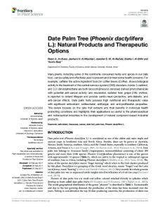
spirals, or contact parastichies, formed by sequences of adjacent organs composing the structure (see Figure 2). Curiously, the numbers of parastichies running in opposite directions are usually two consecutive Fibonacci numbers. The difference between age indexes of two neighboring organs in the parastichy spiral indicates the number of parastichy spirals.

64

56

72

43

48

51

35 40

14 32

66

19

6

59

30

22

27

53

80

38 9

17

1

25

46

67 88

4

45

33

12

11 24

79

3 37

92 29

8 21

54 75

20 7

16

41

2 13

5

62

28

15 10

The palm tree was chosen because of its economic importance and possible future practical implementations. There are two species of the palm family which have economic importance, the oil palm and the date palm. Palm oil is now the most widely produced vegetable oil in the world, demand for which is expected to climb even further as one of the raw materials for biodiesel. The date palm is one of the most important economic tree crops that thrive in the desert regions of the world. In order to reduce labour costs and the risk of working at the top of the palm trees, a number of robotic prototypes for maintenance of palm trees were developed (Aracil et al., 1999; Ripin et al., 2000; Shamsi, 1998). This study proposes a further step in that it will include automatic vision algorithms to guide these robotic systems.

49 23

18

101

neighboring, leaves. The 3D reconstruction is done using the tree model parameters and the location of the leaves on the 2D image.

36 70

31 68 60

44

57

52

Figure 2: The apical meristem of A Norway spruce (Picea abies) (Electron micrograph from (Rutishauser, 1988)). Primordia are numbered according to their age - the higher the number, the older the primordium. Three of the eight right parastichies spirals are illustrated in green, two of the thirteen left parastichies spirals are illustrated in purple. The divergence angle between primordia six and seven which is equal to the Fibonacci angle is marked in the center.

While phyllotactic order is common in the arrangement of seeds in flowers and leaves around a stem, the branching of the trunk and branches is almost unpredictable. In contrast to other trees, both date and oil palms do not have branched trunks, rather incorporating a single, non-branching, trunk with leaves arranged in spiral phyllotactic order its entire length. This simple and consistent arrangement makes it possible to describe these trees by means of a simple model. The proposed algorithm uses the aforementioned model to reconstruct a 3D image of the tree. It receives as input a single image of the date palm. Upon image acquisition, the algorithm proceeds to search for, and locate, the trunk followed by a few prominent leaves. From the location of the prominent leaves the algorithm calculates tree model parameters, which are then used to search for additional,

2

RELATED WORK

The challenging problem of 3D reconstruction of trees has been studied in (Shlyakhter et al., 2001; Martinez et al., 2004). A number of calibrated images from different views of the tree are segmented into the tree, and the background. The background segments are discarded and the tree segments are then compiled to reconstruct a 3D model resembling the specific tree. The target of these works was rendering trees in virtual environments, whereas in our work we try to measure the tree skeleton from only one non calibrated image. Segmentation in these works is done either manually (Shlyakhter et al., 2001), or for cases where the tree background is distinct, such as sky background (Martinez et al., 2004). More sophisticated tree segmentation is done using 51 values measured at each pixel in (Haering and da Vitoria Lobo, 1999). In a recent study (Teng et al., 2006) trunk structure is extracted. The main challenge in this work is to deal with the general trunk structure. In our case however, the trunk is cylindrical. Phyllotactic models are used in the field of computer graphics for simulating realistic plant images. An overview of these models is presented in Section 3. In a recent study (Kaewapichai et al., 2007) the phyllotactic model was used to fit the arrangement of the scales on a pineapple.

3

PALM TREE MODEL

Several mathematical phyllotactic models were developed by computer graphics researchers for the purpose of simulating realistic plant images. Synthesized images of plant structures with predominantly flat, elongated or spherical geometry were created in (Prusinkiewicz and Lindenmayer, 1990; Fowler et al., 1989; Lintermann and Deussen, 1999) using three models: the planar model, the cylindrical model, and the spherical model. These models relate phyllotaxis to the packing problem of equally-sized organs. Many phyllotactic plants do not fit into these models. Phyllotactic plants with a variety of organ sizes and surface shapes were dealt with in (Fowler et al., 1992). In this model plant organs are procedurally placed on the plant’s surface. The palm tree has a spiral phyllotactic pattern. Characteristics of the date palm phyllotaxis have been studied in (Elhoumaizia et al., 2002; Ferry, 1998). In (Elhoumaizia et al., 2002) it was found that the divergence angle of consecutive leaves is similar for the same cultivar and is approximately the Fibonacci angle of 137.5◦ . The handedness of the date palm is the direction in which the leaves are born, clockwise or counter clockwise. The frequencies of right or left handedness in this study were more or less equal. Oil palm measurements, testing for the vertical distance between consecutive leaves, was measured in (Rees, 1964), showing that the horizontal distance between leaves changes only gradually along the length of the trunk. The arrangement of the stubs of pruned leaves on the trunk of the palm tree can be modelled accurately by the cylindrical model. Arrangement of the leaves on the tree crown, on the other hand, deviates from the cylindrical model because the radius of the trunk on the crown decreases. In this paper we used the cylindrical model with adaptations allowing for changes in the trunk’s radius. This model is relatively accurate, while maintaining simplicity and offering an analytical solution.

3.1

Mathematical Model Description

The mathematical model of the palm tree describes both leaf growth locations and leaf growth angles, on the trunk. Leaf growth locations are described in cylindrical coordinates (θ, r, H) with respect to the trunk, where θ is the angle, r is the radius, and H is the height. Leaves are numbered according to their age. The youngest leaf, situated at the top of the tree, is marked as number 1 with consequent leaves being marked according to the order of descent along the

Figure 3: Model of the “skeleton” of the palm tree created using the mathematical model.

tree trunk. The earlier the leaf budded - the higher the number assigned to that specific leaf. Being a leafing plant, the phyllotactic order of the palm tree is not perfect, but still the location of the leaf can be predicted quite accurately from the location of its neighbour. Therefore, the phyllotactic model is defined recursively. The location of leaf number n + i can be calculated from the location of leaf n by the following equations: θn+i = θn + i · h · ψ table

(1)

rn+i = R (n + i) · R Hn+i = Hn − i · d

(2) (3)

αn+i = αtable (n + i)

(4)

where: • h - The handedness of the date palm, 1 for clockwise, -1 for counter clockwise. • ψ - The Fibonacci angle of 137.5◦ . • Rtable ( j) - A table with the ratio of trunk radius at the growing point of leaf number j, to the radius of the trunk at its widest point, R. The table was measured from a reference tree assuming that this value is representative. • d - The vertical distance between two consecutive leaves. • αn+i - Leaf growing angle for leaf number n + i. • αtable ( j) - A table with leaf growth angles for leaf number j. The data was acquired from a reference

tree by measuring images taken from a perpendicular angle to the leaf. Only two parameters are unique for every tree, the handedness of the tree h and the vertical distance between two consecutive leaves d. Knowing these parameters, the location of one leaf, and its age index, we can predict the locations of its neighbors. All values are computed proportional to the radius of the tree whose value can not be recovered from the image. Figure 3 shows a model of the palm tree created using the aforementioned mathematical model. The mathematical model describes a spiral phyllotactic pattern, which can have different parastichy numbers according to r and d. But still for most date palm cultivars, including the one considered here, the parastichy numbers are 5 and 8 (Figure 4). Another assumption of our model is that the leaves grow outward from the axis of the trunk. In other words the leaf midribs are located on a plane containing the trunk axis and the leaf growing point (see Figure 5).

4

ALGORITHM DESCRIPTION

An overview of our proposed algorithm is summarized above. The different stages are summarized in the following subsections and the output of each stage is illustrated in Figure 6. The input of the algorithm is an image of a palm tree, Figure 6(a) is an example of such an image. • Calculating a per pixel probability image of the leaves and trunk (Figure 6(b), Subsection 4.1). • Searching for the location of the trunk and “tree center” using the aforementioned images (Figure 6(c), Subsection 4.2). • Creating, using the leaf probability image and the “tree center”, a leaf clues image (Figure 6(d), Subsection 4.3). • Search for prominent leaves using the leaf clues image (Figure 6(e), Subsection 4.4). • Estimation of the model parameters by using the location of the prominent leaves and their growth angles (Figure 6(f), Subsection 4.5). • Search for more leaves using prediction based on the model parameters (Figure 6(g), Subsection 4.6).

(a)

(b)

Figure 4: Contact parastichy pattern for (a) right handed tree and (b) a left handed tree.

Figure 5: Leaves grow outward from the axis of the trunk.

• 3D reconstruction of the palm tree is achieved by use of the tree model parameters and the location of the leaves on the 2D image (Figure 6(h), Subsection 4.7).

4.1

Calculating Probability Image of the Leaves and Trunk

The interesting part of the leaf of the date palm is its midrib - the central “spine” of the leaf. These midribs and the trunk are the tree’s “skeleton”. The leaflets can be added easily to this “skeleton”, creating a complete model of the tree. The prominent feature of the leaves is their green color, while the distinctive feature of the midrib is its smoothness - low level of gradient. Generating the leaf midrib probability image Pl , denoted as the “leaf probability image”, is based on simple histogram learning techniques described in (Jones and Rehg, 2002). Midrib and non-midrib histograms were collected using a training set of manually labelled images. Given these histograms a four dimensional table with the probability that a given color and gradient defines the leafs’ midrib is calculated (see Figure 7). The table is applied to the original image to get the leaf probability image. The size of the histogram is 30 bins/channel for the HSV channels, and 10 bins/channel for the gradient. In practice,

(a) Original image.

(e) Prominent search.

leaves

(b) leaf and trunk proba- (c) Trunk location and bility images. “tree center”.

(f) Model prediction.

(g) Search leaves.

for

more

(d) Leaf clues image.

(h) VRML 3D model.

the combination of color and smoothness has proved to be both informative and robust. The dominant feature of the trunk is its color. The trunk probability image - Pt is calculated in the same way as the leaf probability image only without considering the gradient. The leaf and trunk probability images are illustrated in Figure 6(b) in green and blue respectively.

4.2

Value

Figure 6: Output of algorithm stages. (e)-(g) show a zoomed in section of the original image.

Search for Trunk Location and “Tree Center”

The location of the trunk is represented by three parameters: the horizontal location on the image in pixels - x, trunk radius in pixels - r, and the leaning angle of the trunk toward the camera - γ (see Figure 8(a)). Assuming that the image was taken nearly parallel to the horizon, and that the palm trunk is perpendicular to the ground, knowing these three parameters, enables the calculation of the 3D location of the trunk, and the transformation between location on the 3D trunk to the image and vice versa. We define the tree center as the point on the line of symmetry of the trunk, with the vertical location on the image in pixels - y, immediately beneath the oldest leaf (see Figure

Sa tu

ra t ion

Hue

Figure 7: 3D “slice” of the 4D leaf probability table, defines the probability of a given color with gradient size: 6-8. The probability is illustrated by a ball whose size is proportional to the probability.

8(a)). We call it the tree center because it is almost the intersection point of all the leaves midribs line. The tree center will be used later for the removal of leaf

clues not in the direction “intersecting” with the tree center. Estimation of the four trunk location and tree center parameters (x, r, y, γ) is done by searching for the best location of a schematic model of the tree on both the trunk and the leaf probability images. The model is illustrated in Figure 8(b). Assuming that γ is not too large, the trunk can be represented by a vertical rectangle on the image plane. The “trunk rectangle” is separated into two rectangles, D - descending and U - ascending from the common “tree center”. Rectangles R and L represent the outer border of the trunk, an area that should have pixels with low probability in the trunk probability image. A leafy area is represented by rectangle M which should have a high probability for pixels in the leaf probability image. The location and size of these rectangles are functions of x, r and y. For performance reasons the search is done in phases. The first phase searches horizontally for x and r, using the “Integral Image” algorithm (Viola and Jones, 2001) it maximizes the energy function: 1

Eh (x, r) = ( f (U ∪ D, Pt ) − f (L, Pt ) − f (R, Pt )) · r 3 , (5) ∑

(i, j)∈A

P(i, j)

where f (A, P) = i, j kAk represents the average probability of the pixels in the rectangle A on the 1 probability image P. The term r 3 was added to prevent very thin trunks from being accepted. For every local maximum a search for y is done using pattern search (Lewis and Torczon, 2000) by maximizing: Ev (x, r, y) = ( f (M, Pl ) + f (D, Pt ) − f (U, Pt )). (6) The best (x, r, y) combination is chosen by maximizing: E(x, r, y) = Ev (x, r) · Eh (x, r, y). (7) Finally the best γ is chosen. Both left and right trunk line-boundary angles are searched for in order to maximize the derivative over the trunk probability image. The intersection point of these lines is used in order to calculate γ. Results of the search for trunk location and tree center are illustrated in Figure 6(c). The tree center is marked by a white cross, and the trunk borders are drawn in magenta.

4.3

Creating the Leaf Clues Image

The leaf clues image is created from the leaf probability image - Pl by thresholding. After thresholding, groups of connected pixels that we call leaf clues remain. The dominant clue direction is calculated using PCA. Clues whose extensions do not intersect with a circle around the tree center (whose radius is 32 · r) are removed. Figure 6(d) shows an example of a leaf clues image, with the tree center marked.

U

M L

R

y

γ

x

D

r (a)

(b)

Figure 8: (a) Trunk location and “Tree Center” parameters description. (b) Rectangles U, D, R, L, and M, used in the search for the trunk location and “Tree Center”.

4.4

Search for Prominent Leaves

The purpose of prominent leaf search is to find enough leaves to be able to calculate the model parameters. Figure 6(e) illustrates the result of this search. The leaf search is done on the leaf clues image from bottom up because the lower leaves (older) always hide the younger leaves above them. Only the frontal leaves are considered because they are more prominent and distinct. The process is iterative and includes three parts: locating the leaf’s start point in the leaf clues image, tracking this leaf from its start point, and removing the leaf found from the leaf clues image and the leaf probability image. These parts are explained below. Locating the Leaf Start Point: The leaf start point is chosen as the lower point of a clue in the leaf clues image. The clue is chosen from a region in the center of the trunk, above the tree center. Tracking the Leaf: The leaf is tracked from its growing point using the leaf probability image and the original image in HSV color space. Tracking is done using segments whose length is one third of the trunk’s radius. The end of each segment is the beginning of the following segment but in a different direction (Figure 9). The width and length of every segment is calculated according to the model and the leaf starting point. The tracking is done using a particle filter (Arulampalam et al., 2002), with a weight function which is the product of the following terms: • Sum of leaf pixels on the leaf probability image plus the number of pixels that belong to this specific clue in the proposed leaf. This encourages the leaf model to be on the leaf pixels and on the starting clue (illustrated in green in Figure 9). • 1/sum of the standard deviations of the pixels

along the lines of the leaf segments (illustrated by the blue lines in Figure 9). This discourages crossing over to other leaves because lines along a leaf tend to be smooth. • Number of pixels of the proposed leaf that are not sky pixels. A simple definition for a sky pixel in HSV color space was determined empirically. • 1/sum of the ascending angles. Consider the angles between successive leaf parts, illustrated in Figure 9 as β1 − β5 . Ascending angles are defined as negative angles. They are counted to discourage the leaf from ascending against gravity. Leaf samples are propagated by adding segments with the mean direction of the previous segment pertubrated by Gaussian noise with σ = leaf radius relative 4 to the end of the segment. β3

β4

β5

β2

β1

Figure 9: Particle filter tracking model.

Removing the Leaf: Once the geometric shape of the leaf has been found, it is removed from leaf clues image and the leaf probability image.

4.5

Estimating Model Parameters

The exact location of neighboring leaves depends on the leaf parameters and the tree model equations. Nevertheless, parameter similarities between trees give similar parastichy patterns, making it possible to estimate the location of a neighboring leaf while accounting for the handedness (possible locations are calculated by using a range of possible parameters). The first step in model parameter estimation is done twice; once for the possibility of right handedness and once for left handedness. Leaves found in the last step are matched into a list of neighboring couples according to their relative location. d is calculated for every couple from the location of the two leaves according to Equation 3. From the list of the d’s outliers are removed and the handedness of the tree is chosen to be the one with the most inliers and d is computed as the mean value of the inliers. The relative age index between leaf couples is known according to their relative location and handedness. All leaves are numbered according to their

age index in relation to the lowest leaf. The leaf index of the lowest leaf is chosen as the one with the minimal sum of differences between the leaf angle as seen in the image in relation to the prediction of the leafs’ angle according to the model using the projection of α from Equation 4 on to the image. Figure 6(f) is the tree image. Prominent leaves are marked in green with their age indexes, while those marked in magenta predict the location and angle of other leaves according to the model.

4.6

Search for More Leaves

Model parameters and prominent leaf age indexes enable the prediction of neighboring leaf locations and growth angles using the tree model equations. The search for more leaves is done iteratively by searching for neighboring leaves from the bottom up. Every tree location and growth angle of neighboring leaves is calculated. If a leaf clue exists in the leaf clue image in that area, then leaf tracking is performed in the same way as in Section 4.4. After the search a leaf is accepted if the percentage of pixels in the geometric shape of the leaf, found in the leaf clue image, is beyond a given threshold. Figure 6(g) illustrates the result of this search. All the leaves found, including the ones found in the search for the prominent leaves are marked in magenta.

4.7

3D Reconstruction

As mentioned in Section 3.1, one of the assumptions of the tree model is that the leaves grow outward from the axis of the trunk. Using this assumption, knowing the location of the trunk and the location of the leaf midrib on the 2D image and including the leaf growing point, we are able to calculate the location of the 3D midrib. Figure 6(h) is a 3D VRML model of the date palm tree based on these calculations.

5

EXPERIMENTS

The algorithm described in this paper has been implemented in MATLAB and tested on nearly 50 images of date palm trees. In the first stage the leaf, trunk and sky probability image were generated from a small number of manually labeled images. The radius table Rtable ( j) and the leaf angle table αtable ( j) were measured from a small set of images of a tree. Several results of the execution of the algorithm are presented in Figure 10. Additional results as well as the VRML models can be viewed at: http://mis.hevra.haifa.ac.il/∼ishimshoni/Phyllotaxis/ .

6

CONCLUSION AND FUTURE WORK

In this paper, we proposed a new 3D reconstruction algorithm which reconstructs the 3D model of the date palm tree from a single uncalibrated input image by using the spiral phyllotactic pattern. To demonstrate the effectiveness of the proposed method, we show several output VRML model images. 3D reconstruction from a single input image is, naturally, only the first step in the development of automatic vision algorithms to guide autonomous palm tree maintenance machines. We envision the next step to be the further development of the algorithm by incorporating structure from motion techniques in order to improve the accuracy of the algorithm and to integrate the algorithm into a robotic prototype. The proposed algorithm can also be applied to additional phyllotactic plants.

REFERENCES Adler, I., Barabe, D., and Jean, R. (1997). A history of the study of phyllotaxis. Ann. of Botany, 80(3):231–244. Aracil, R., Saltar´en, R., and Sabater, J. (1999). Trepa: Parallel climbing robot for maintenance of palm trees and large structures. In Proc. of Int. Workshop and Conf. on Climbing and Walking Robots, pages 453–461. Arulampalam, M. S., Maskell, S., Gordon, N., and Clapp, T. (2002). A tutorial on particle filters for online nonlinear/non-gaussian bayesian tracking. IEEE Transactions on Signal Processing, 50:174–188. Atela, P. and Gol´e, C. (2008). Phyllotaxis - an interactive site for the mathematical study of plant pattern formation. www.math.smith.edu/∼phyllo/. Cummings, F. W. and Strickland, J. C. (1998). A model of phyllotaxis. J. of Theo. Biology, 192(4):531–544. Elhoumaizia, M. A., Lecoustreb, R., and Oihabic, A. (2002). Phyllotaxis and handedness in date palm (phoenix dactylifera l.). Fruits, 57(5-6):297–303. Ferry, M. (1998). The phyllotaxis of the date palm (phoenix dactylifera l.). In Proc. Inter. Conf. on Date Palms, AlAin, UAE, pages 559–571. Fowler, D. R., Hanan, J., and Prusinkiewicz, P. (1989). Modelling spiral phyllotaxis. Computers and Graphics, 13(3):291–296. Fowler, D. R., Prusinkiewicz, P., and Battjes, J. (1992). A collision-based model of spiral phyllotaxis. In Proc. ACM Conf. on Computer Graphics and Interactive Techniques, pages 361–368. Haering, N. C. and da Vitoria Lobo, N. (1999). Features and classification methods to locate deciduous trees in images. Comp. Vis. and Im. Under., 75(1-2):133–149. Jean, R. V. (1994). Phyllotaxis: a systemic study in plant morphogenesis. Cambridge University Press.

Jones, M. J. and Rehg, J. M. (2002). Statistical color models with application to skin detection. International Journal of Computer Vision, 46(1):81–96. Kaewapichai, W., Kaewtrakulpong, P., Prateepasen, A., and Khongkraphan, K. (2007). Fitting a pineapple model for automatic maturity grading. In ICIP, pages I: 257– 260. Lewis, R. M. and Torczon, V. (2000). Pattern search algorithms for linearly constrained minimization. SIAM Journal on Optimization, 10(3):917–941. Lintermann, B. and Deussen, O. (1999). Interactive modeling of plants. IEEE Computer Graphics and Applications, 19(1):56–65. Martinez, A. R., Mart´ın, I., and Drettakis, G. (2004). Volumetric reconstruction and interactive rendering of trees from photographs. ACM Trans. Graph, 23(3):720–727. Prusinkiewicz, P. and Lindenmayer, A. (1990). The Algorithmic Beauty of Plants. Springer-Verlag. Rees, A. R. (1964). The apical organization and phyllotaxis of the oil palm). Annals of Botany, 28:57–69. Reinhardt, D. (2005). Regulation of phyllotaxis. International Journal of Developmental Biology, 49(5/6):539–546. Ripin, Z. M., Soon, T. B., Abdullah, A. B., and Samad, Z. (2000). development of a “low cost” modular pole climbing robot. TENCON, 1:196–200. Rutishauser, R. (1988). Symmetry in Plants, chapter Plastochron ratio and leaf arc as parameters of a quantitative phyllotaxis analysis in vascular plants, pages 171– 212. World Scientific Publications. Shamsi, M. (1998). Design and development of a tree climbing date harvesting machine. PhD thesis, Silsoe College, Cranfield University, UK. Shlyakhter, I., Rozenoer, M., Dorsey, J., and Teller, S. (2001). Reconstructing 3D tree models from instrumented photographs. IEEE Computer Graphics and Applications, 21(3):53–61. Smith, R. S., Guyomarc’h, S., Mandel, T., Reinhardt, D., Kuhlemeier, C., and Prusinkiewicz, P. (2006). A plausible model of phyllotaxis. Proceeding - National Academy of Sciences USA, 103(5):1301–1306. Steeves, T. A. and Sussex, I. M. (1989). Patterns in plant development. Cambridge University Press. Teng, C. H., Chen, Y. S., and Hsu, W. H. (2006). An approach to extracting trunk from an image. IEICE Transactions, E89-D(4):1596–1600. Viola, P. and Jones, M. (2001). Rapid object detection using a boosted cascade of simple features. In Proceedings CVPR, pages I:511–518.

Original images

Segmented leaves Figure 10: Results of the algorithm’s operation

VRML 3D model