Using pipeline information in a multi-echelon spare parts inventory system Christian Howard, Ingrid Reijnen, Johan Marklund, Tarkan Tan Beta Working Paper series 330
BETA publicatie ISBN ISSN NUR Eindhoven
WP 330 (working paper) 978-90-386-2372-6 804 September 2010
Using pipeline information in a multi-echelon spare parts inventory system Christian Howard ● Ingrid Reijnen ● Johan Marklund ● Tarkan Tan Department of Industrial Management and Logistics, Lund University Department of Industrial Engineering and Innovation Sciences, Eindhoven University of Technology
[email protected] ●
[email protected] ●
[email protected] ●
[email protected]
Motivated by collaboration with a global spare parts service provider, we consider a two-echelon inventory system with multiple local warehouses, a so-called support warehouse, and a central warehouse with ample capacity. In case of stock-outs, the local warehouses can receive emergency shipments from the support warehouse or the central warehouse at an extra cost. The focus is on using information on orders in the replenishment pipeline, i.e. pipeline information, to achieve cost efficient policies for requesting emergency shipments. We introduce a policy where the request for an emergency shipment is based on the time until an outstanding order will reach the stock point considered. The goal is to determine how long one should wait for stock in the replenishment pipeline, before requesting an emergency shipment, and the cost effects of using pipeline information in this manner. In our analysis we utilize results from queuing theory and provide a decomposition technique that reduces a complex multi-echelon problem to more manageable single-echelon problems. Our results indicate that there is a significant benefit in using pipeline information. Based on data provided by the case company, we illustrate that the relative cost increase of ignoring pipeline information can be as high as 106%.
Keywords:
Emergency shipments, Inventory, Multi-echelon, Pipeline information, Spare parts
1. Introduction The cost of downtime resulting from failed equipment and waiting for missing spare parts is a major concern for many companies. The research presented in this paper is motivated by collaboration with Volvo Parts Corporation, a global spare parts service provider with headquarters in Sweden. Volvo Parts is the supplier of aftermarket services for the Volvo Group, supporting the business areas: Volvo Trucks, Mack, Renault Trucks, Volvo Busses, Volvo Heavy Machinery and Volvo Penta. It follows that the core operational area for Volvo Parts is stock keeping and distribution of spare parts. These spare parts are distributed through central warehouses, positioned around the world, each one
1
responsible for serving several local markets. On each local market they have a number of local warehouses (dealers/retailers) that, in turn, serve the end customer. This includes both service and repairs of the customers’ vehicles, as well as direct “over the counter” sales of the spare parts. The local warehouses replenish their stock by placing orders at the central warehouse. A vehicle that is idle in the workshop due to a parts failure directly results in lost revenue for Volvo Parts’ customer, and this leads to a demand for high availability of spare parts at the local warehouse responsible for repairing the vehicle. To achieve this high availability, Volvo Parts combines regular stock replenishments from the central warehouse with emergency shipments. That is, a stock-out situation at a local warehouse is often resolved by sending an extra shipment from a source that does have the spare part in stock. Therefore, on most local markets, they have an additional stock point, referred to as a support warehouse. The support warehouse is also replenished by the central warehouse and its purpose is to provide these emergency shipments to the local warehouses in cases of stock-outs. The shipments are much faster than regular replenishments, but they come at higher cost. As a last resort, the central warehouse can also provide an emergency shipment to the local warehouse, should the support warehouse be out of stock as well. This type of system structure is by no means unique for Volvo Parts. It is, for instance, also utilized by some of their competitors. At Volvo Parts, the general policy is to ask for an emergency shipment whenever a stock-out occurs. However, as recognized by the company, this is not necessarily the best strategy in terms of cost and service efficiency. For some spare parts it might be better to backorder the demand at the given stock point, in anticipation of the next incoming regular order, instead of requesting an emergency shipment. In particular, if there is a regular replenishment order from the central warehouse in close proximity to the local warehouse, the customer might actually receive the part sooner if she waits for this incoming shipment. At the same time Volvo Parts avoids the extra cost associated with an emergency shipment. This highlights the need for a replenishment policy that is more flexible regarding the use of emergency shipments, and that utilizes information on when outstanding orders in the replenishment pipeline from the central warehouse will be arriving. We refer to this as using pipeline information. In this paper, we focus on a single local market and introduce a tolerance time for backordering customers. This tolerance time can be set individually for each product and stock point in the system and is designed to incorporate the possibility of waiting for incoming replenishment orders. When demand occurs at a specific local warehouse, and that warehouse is out of stock, the demand is backordered if there is a regular replenishment order arriving within the set tolerance time. If there is no regular order close enough in the pipeline, an emergency shipment is requested. The request first goes to the support warehouse which will meet the demand and send an emergency shipment if there is stock on hand or stock arriving within its own tolerance time. If this is not the case, the local warehouse requests an emergency shipment from the central warehouse instead. We assume that the
2
central warehouse always can deliver and therefore, for the purpose of this work, it can be viewed as an external supplier. Hence, the multi-echelon nature of the model that we consider is derived from the support warehouse (upper echelon) supplying the local warehouses (lower echelons) with emergency shipments. Our model assumes Poisson distributed customer demand and base-stock, or (S-1,S), policies at all stock points, which is reasonable for the slow moving items in Volvo Part’s product assortment. Moreover, we consider a customer waiting cost (e.g. based on loss of goodwill and penalty costs stipulated in service contracts etc.) per unit and time unit. Given this waiting cost, along with holding costs per unit and time unit and emergency shipment costs per unit, we provide a method for determining base-stock levels and tolerance times such that the expected system costs are minimized. One of the main advantages with our model is that when all tolerance times are set to zero this corresponds to the current situation at Volvo Parts, where emergency shipments are used whenever a stock-out occurs. Conversely, if all tolerance times are equal to the replenishment lead time, all demand will wait for regular replenishment and emergency shipments are never used. Our model can therefore provide structural results on suitable system configurations for different products (i.e. for which products should emergency shipments be used?), which is a key interest point for Volvo Parts. Numerical results based on data provided by Volvo Parts show that the penalty, i.e. the relative cost increase, of ignoring pipeline information and always requesting an emergency shipment can be as high as 106%. The remainder of the paper is organized as follows: Section 2 provides a review of related literature. Section 3 presents the considered model in detail and discusses the assumptions made. Section 4 analyzes a single local warehouse in isolation and provides an exact method for cost evaluation and optimization of this single-echelon system. Based on these results an accurate heuristic for setting base-stock levels and tolerance times for all local warehouses and the support warehouse is presented. Section 5 evaluates the performance of the heuristic and provides managerial insights into the value of using pipeline information, both in the single - and multi-echelon case. Section 6 concludes.
2. Literature review There are obvious connections between our work and the literature on lateral transshipment, dual supply, partial backordering, and multi-echelon systems. The lateral transshipment literature focuses on models where locations in the same echelon can share inventory by transferring items between the locations. Dual supply models analyze situations where a stock point can have more than one supplier to choose from, e.g., a regular supplier and an emergency supplier. The partial backordering literature is concerned with inventory policies that allow backordering under certain conditions, e.g., by setting
3
a maximum number for the amount of customers that can be backordered. Multi-echelon models focus on systems with multiple levels, where an upper level supplies the lower levels. For a recent overview of the lateral transshipment literature we refer to Paterson et al. (2009) and Wong et al. (2006). We particularly mention the papers by Kranenburg and van Houtum (2009) and Reijnen et al. (2009) because, similar to a support warehouse, they have designated suppliers of transshipments. Kranenburg and van Houtum consider a two level structure where lateral transshipments can only be supplied by the upper level. Reijnen et al. consider a structure where local warehouses can only receive a lateral transshipment from another local warehouse if the local warehouse can be reached within a predefined time limit. However, even though the authors of both papers recognize that the lateral transshipment time is non-negligible, they do not consider waiting for a replenishment order in the pipeline as an alternative to sending an emergency shipment. A lateral transshipment model that incorporates the option of waiting for incoming orders is Yang and Decker (2010). They consider a structure similar to Reijnen et al. where it is assumed that customers are willing to wait at a local warehouse for a given amount of time. Here, a local warehouse will wait for incoming orders, instead of requesting a lateral transshipment, if the order will arrive within this given time limit. This is similar to our assumptions but there are important differences. Firstly, they regard the customer time limit as a given parameter and assume that the customer is satisfied if she receives the item within this time (which makes it similar to a service constraint). Although our tolerance times could be used in a similar way, we assume a customer waiting cost per time unit at each local warehouse and regard the time one should wait as a decision variable in our policy. Secondly, they place the restriction that all local warehouses have the same time limit, whereas we allow for different tolerance times at different locations. Lastly, in their work they assume that demand is backordered if no lateral transshipment can reach the local warehouse in time, while we consider an emergency shipment from the central warehouse as a last option. These differences mean that we use fairly unrelated methods of analysis. Axsäter (2003a) suggests a heuristic decision rule for lateral transshipments that incorporates the remaining delivery times for outstanding orders. Although we also utilize this information, our use of tolerance times is quite different from Axsäter’s transshipment rule. Furthermore, we place an emphasis on determining replenishment policy parameters, whereas Axsäter uses simulation for cost evaluation and optimization of (R,Q) policies under the given transshipment rule. Our work is also related to the literature on unidirectional lateral transshipment models (see e.g. Axsäter, 2003b and Olsson, 2009) because the emergency shipments exclusively occur in one direction (from the support warehouse to the local warehouses). The distinguishing feature with our work is that we consider the inventory in the pipeline before requesting an emergency (lateral) transshipment. Even though most papers recognize that there is some lateral transshipment lead time, they do not consider waiting for a replenishment order as an alternative to an emergency (lateral) transshipment.
4
Another paper with an obvious relation to our current work is Axsäter et al. (2010), which also analyzes the described distribution system used by Volvo Parts. However, their work is focused on minimizing costs under fill rate service constraints and, therefore, they do not consider the customer waiting times explicitly. Moreover, they do not consider pipeline information, and their model assumes that the local warehouses always order from the support warehouse when a stock-out occurs. An emergency shipment from the support warehouse can also be viewed as a delivery from a second supplier, implying a connection between our present work and that on dual supply models. In these models a single stock point has the option of using a second supplier that can deliver emergency shipments at an extra cost. The main difference, compared to our work, is that the emergency supplier is exogenous, while we include the support warehouse in our model. In the analysis of a single local warehouse in Section 4 we explore the differences and similarities to a dual supplier model analyzed by Moinzadeh and Schmidt (1991), and Song and Zipkin (2009). For a more extensive overview on dual supply models we refer to Minner (2003). The third stream of literature that shares similarities with our work is that of partial backordering. In our model, a customer that waits for a regular replenishment to arrive is regarded as a backordered customer. Basing the decision to backorder on a tolerance time can therefore be viewed as a type of partial backordering. For partial backordering models concerning (S-1,S) policies and Poisson demand we refer to Das (1977) and Moinzadeh (1989) and references therein. What sets this literature apart from our current work is the focus on single-echelon models and the fact that partial backordering is the result of a given customer behavior, i.e. that customer are willing to wait for a certain amount of time before leaving the system. Therefore, the modeling techniques are different and these papers do not investigate the value of being able to choose when to backorder a demand. Models that do investigate the value of partial backordering are given in Chu et al. (2001) and Rabinowitz et al. (1995). They study a single-echelon system under Poisson demand where customers are backordered when a replenishment order is close enough in the pipeline. Although they illustrate that there is a large potential in allowing for partial backordering, their analysis assumes (R,Q) replenishment policies under the assumption that there can be at most one order outstanding. In many cases, when allowing for backorders, this assumption is likely to be violated and, hence, the analysis is approximate in these cases. The focus on a two-level system with a single stock point in the upper echelon supplying multiple downstream facilities implies that there is a relation between our current work and the literature on continuous review distribution systems. Although there are some similarities, the main difference is that the support warehouse in our model handles emergency shipments, whereas the upper echelon in previous literature typically handles regular replenishment orders. As a result, the problem formulations and solution techniques differ. For a general overview of the literature on distribution systems we refer to Axsäter (2003c). A more recent overview of the literature on
5
continuous review one warehouse multiple retailer systems is available in Axsäter and Marklund (2008).
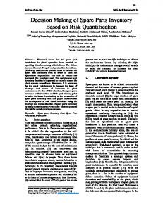
3. Problem formulation We consider a single item inventory model consisting of j local warehouses (index j {1,…,J}), a support warehouse (index j = 0), and a central warehouse with infinite capacity (Figure 1). All stock points apply continuous review base-stock, or (S-1,S), policies and the customer demand at local warehouse j follows a Poisson process with demand rate λj. These assumptions are reasonable for the slow moving spare parts in Volvo Parts assortment. Demand is satisfied according to a First ComeFirst Serve (FCFS) rule.
Figure 1 For fulfillment of a demand we first consider the stock on hand and the orders in the replenishment pipeline (i.e. outstanding orders on route from the central warehouse) at local warehouse j, where the demand occurred. In case local warehouse j has available stock on hand, the customer leaves directly with an item. If the warehouse is out of stock and an unreserved replenishment order will arrive within Tj time units, then the demand is backordered and waits until the order arrives. By unreserved we mean that there is no other customer demand backordered and waiting for the considered item. We refer to the decision variable Tj as the tolerance time at warehouse j. In case a customer demand is satisfied from stock on hand or backordered at local warehouse j a new item is ordered from the central warehouse with constant lead time Lj, at the moment the demand occurs. If there is no stock on hand, or in the replenishment pipeline that will arrive within the tolerance time, then that demand will
6
be satisfied by an emergency shipment. A demand waiting for an emergency shipment at a local warehouse is not viewed as a backorder at that stock point. This is because the responsibility for fulfillment of that demand is now shifted to the support warehouse and the central warehouse. When requesting an emergency shipment, the local warehouse first contacts the support warehouse which applies the same policy: (i) satisfy the demand from stock on hand by sending a shipment to the local warehouse straight away, (ii) backorder the demand based on the pipeline inventory of reach within tolerance time T0 and send a shipment when the item arrives in stock, (iii) deny the request for an emergency shipment. In case (iii), the local warehouse requests an emergency shipment from the central warehouse, which can always deliver. We assume that all emergency shipment lead times (including picking, packing, shipping and receiving) are constant, but they may vary between local warehouses. In the case of emergency shipments from the support warehouse, the time for waiting on items in the replenishment pipeline is not included in this lead time. Let c j
s j
and
be the lead times for emergency shipments to local warehouse j, from the support warehouse and
central warehouse, respectively. It follows that the maximum waiting time for a customer arriving at local warehouse j is given by max(Tj, T0 +
s j
,
c j
). Note that this holds for the case when T j < Lj and
T0 < L0. In the special case of Tj = Lj we have complete backordering at local warehouse j and the maximum waiting time is therefore Tj. Similarly, if T0 = L0 and Tj < Lj the maximum waiting time is given by max(Tj, T0 +
s j
), because emergency shipments from the central warehouse will never be
used. The relationship with the maximum waiting time means that the tolerance times can be set to fulfill a given customer service requirement. It is, for instance, common to have service contracts where a spare part is guaranteed to be delivered within a certain time limit. Another approach is to base the value of the tolerance times on the emergency shipment lead times. For example, with Tj = min(
s j
,
c j
) j {1,…,J} a local warehouse only backorders demand if this guarantees faster
delivery than an emergency shipment, and with T0 =
c j
−
s j
(assuming
c j
s j
) the support
warehouse only backorders demand if this saves time compared to an emergency shipment from the central warehouse. This approach is reasonable if the cost of waiting for a part is so high that choosing the quickest option is the only reasonable approach. However, this is not the case for all spare parts at Volvo Parts. In this work the focus is more general, where the system can choose tolerance times based on what is most cost efficient. This approach implies that we investigate the full potential in using tolerance times. Moreover, it means that we can provide Volvo Parts with a tool for finding the most efficient way of using emergency shipments. We assume a customer waiting cost, bj, per unit and time unit at local warehouse j. This cost can, for instance, be based on loss of goodwill and the cost of downtime for vehicles being serviced.
7
Furthermore, there is a fixed per unit cost, cj, associated with every emergency shipment from the support warehouse to local warehouse j. Analogously, there is a fixed per unit cost, pj, for every emergency shipment from the central warehouse, pj cj. Note that, because we consider constant emergency shipment lead times, the customer waiting costs incurred from waiting on items in transport from the support warehouse (bj
s j
), or the central warehouse (bj
c j
), will be the same for all
customers at local warehouse j. These costs are therefore included directly in cj and pj, respectively. However, waiting due to backordering, either at the support warehouse or a local warehouse, needs to be handled separately. We also consider inventory holding costs hj (j {0,…,J}) per unit and time unit for stock on hand. Let S = (S0, S1,…,SJ) be the vector of the support warehouse and local warehouse base-stock levels, and let T = (T0, T1,…,TJ) be the vector of the tolerance times. We refer to the policy applied at each stock point j as an (Sj,Tj) policy. For demand occurring at local warehouse j (j {0,…,J}) we define: αj
=
fraction of demand satisfied from stock on hand at local warehouse j
βj
=
fraction of demand backordered at local warehouse j
γj
=
fraction of demand satisfied from stock on hand at the support warehouse
δj
=
fraction of demand backordered at the support warehouse
θj
=
fraction of demand satisfied by the central warehouse
ψj
=
γj + δj + θj, i.e., fraction of demand satisfied through emergency shipments
EWj
=
expected waiting time for an item backordered at local warehouse j
EVj
=
expected waiting time at the support warehouse for an item requested at local warehouse j and backordered at the support warehouse
EILj+
=
expected inventory on hand at stock point j.
Note that all customer demand must eventually be satisfied, i.e. αj + βj + γj + δj + θj = 1. The objective is to find the S and T ( 0 Tj J
C(S, T)
L j for all j) that minimize the expected total system cost per time unit: J
h jEIL j j 0
J
bj
j
J
jEWj
j 1
cj j 1
j
j
J j
j 1
b jEVj ) j (c j
pj
j
j
.
(1)
j 1
In (1), the first term is the expected holding costs, the second term is the expected costs for backorders at the local warehouses, the third term is the expected cost for emergency shipments sent immediately from the support warehouse, the fourth term is the expected cost for emergency shipments sent, after a delay, from the support warehouse, and, finally, the last term is the expected cost for emergency shipments sent from the central warehouse. The settings described above correspond well to the current setup of Volvo Parts’ distribution system for low demand spare parts. There is, however, an alternative interpretation of the options of demand fulfillment. From a modeling perspective, we can view the request for an emergency
8
shipment from the support warehouse as demand being lost at the local warehouse, and instantly transferred to the support warehouse. The parameter cj can then be interpreted as the cost of transferring the demand. In the same way, an emergency shipment from the central warehouse can be viewed as demand being lost for the support warehouse at an additional cost pj − cj. We can therefore alternatively rearrange (1) as J
C(S, T)
J
h jEIL j j 0
J
bj j 1
j
J
jEWj
cj j 1
j
J
bj
j j 1
j
jEVj
(p j c j )
j
j
,
(2)
j 1
where the third and fifth terms now are the costs for losing/transferring demand and the fourth term is the costs for backorders at the support warehouse.
4. Analysis This section presents the analysis of the considered model. First, we focus on a local warehouse j in isolation, and show how the costs for a given (Sj,Tj) policy can be evaluated exactly. We then present a method for optimizing these decision variables. Next, utilizing these results, we provide heuristic for cost evaluation and for finding near-optimal values of the decision variables in the multi-echelon system.
4.1 Single-echelon model We focus on a single local warehouse with the aim to determine the expected costs per time unit for a given (S,T) policy. For notational convenience we suppress the index j in this section. Demand is satisfied either directly from stock on hand, after being backordered for at most T time units, or from an emergency shipment. In this context we make no distinction as to where the emergency shipment comes from, only that the entire cost for the emergency shipment can be quantified by the parameter p. The most straightforward interpretation of this is that the support warehouse is removed from the multi-echelon system, thus leaving the central warehouse as the only option for emergency shipments. We can therefore focus solely on the fraction of demand satisfied by emergency shipments, ψ, compared to γj, δj and θj in the multi-echelon model. Note that we can choose to view ψ as the fraction of demand that is lost to the system, at a fixed per unit cost p. A schematic representation of the local warehouse, for a given (S,T) policy, is provided in Figure 2. In Figure 2 we see that the replenishment pipeline can be separated into two parts. The first part is of length (L−T), and an order in this part of the pipeline cannot be reserved by an arriving customer. The second part is of length T, and an (unreserved) order in this part of the pipeline can be reserved for an incoming customer demand. We define the inventory position of the whole system, IP1, as the sum of the inventory level (stock on hand minus backorders), the number of items on order in the first part of the pipeline (denoted by N1), and the number of items on order in the second part of
9
the pipeline (denoted by N2). Note that at any point in time IP1 = S holds. Similarly, we define IP2 as the inventory level plus the number of items in the second part of the pipeline.
IP1 L
IP2
N1
N2
L-T
IL
T
Figure 2 This implies that IP2 = IP1−N1 and that 0 IP2 IP1. Furthermore, it means that a demand can be satisfied at the local warehouse if IP2 > 0 and that demand is lost for the local warehouse (satisfied by an emergency shipment) if IP2 = 0, or equivalently, N1 = S. Following the notation in Section 2, our objective is to find the S and T that minimize the expected costs per time unit C(S, T)
hEIL
b
.
EW p
In subsequent sections we refer to this single-echelon model as the Time Based Backordering (TBB) model.
4.1.1 Cost evaluation for a given (S,T) policy We begin with the trivial case when S = 0. Because there will never be any unreserved items in the replenishment pipeline and all demand will be lost unless T = L we have
C(0, T)
p
;0 T L
b L ;T L
.
The result for S = 0 and T = L (i.e. complete backordering) follows from Little’s law. For the case with S 1, the TBB model can be represented as a queuing network, depicted in Figure 3.
No
Yes Poisson(λ)
N1 S. Analysis of this queuing network is difficult because there is no known product-form solution (and it is unlikely that one exists) to the steady state distribution of the occupancy of the system. However, we will show that this network can be analyzed by utilizing results from a similar queuing network, stemming from slightly different assumptions regarding the fulfillment of customer demand. Therefore, for the moment, assume that a customer facing a stock-out situation is now always backordered (never lost) at the local warehouse and that this always triggers a replenishment order. Furthermore, assume that the local warehouse has the option of choosing between two different suppliers, the first one with lead time L, and the second one with lead time T, T L. The local warehouse always places its orders at the first supplier, unless a stock-out occurs and an order from the second supplier can reach the local warehouse before an (unreserved) order from the first supplier. In this case an order is placed at the second supplier. This situation corresponds to a special case of the so-called “dual index policy” (see e.g. Song and Zipkin, 2009). In its general form, the dual index policy allows for the ordering from each supplier to be based on the two inventory positions IP1 and IP2, respectively, but for our purposes the second supplier is only used when IP2 = 0 and an order arrives. We will refer to this model as the Dual Supply model (DS) model, and it can be described by the queuing network depicted in Figure 4. In the DS model the number of orders in each part of the pipeline is denoted M1 and M2, respectively. No
Yes Poisson(λ)
M1