Using prior-phase effort records for re-estimation during software ...

Using Prior-Phase Effort Records for Re-estimation During Software Projects Stephen G. MacDonell

Martin J. Shepperd

School of Computer and Information Sciences

Empirical Software Engineering Research Group

Auckland University of Technology Private Bag 92006 Auckland, New Zealand [email protected]

School of Design, Engineering and Computing Bournemouth University Bournemouth, BH1 3LT, UK [email protected] Obtaining accurate measures and estimates of project size, effort and duration early in the software process has been a long-term goal of software engineering research and practice. Such measures and estimates are used frequently as the basis of tenders or bids for contract development, for planning systems development and integration activities, and for the ongoing management of these activities as they occur. These tasks all have potential implications for any associated project budget. For instance, a successful bid will have an impact on expected revenue and expenditure; project plans are generally formulated in order to ensure the most efficient use of costly resources (principally labor); and monitoring and feedback during a project can enable adjustments to be made in order to further optimize the performance of the project team and/or the organization as a whole. Given the potentially significant impact on an organization’s revenues and expenditure, and consequently their ability to earn a profit, accuracy in measurement and estimation is highly sought after. In this paper we investigate the potential of re-estimation during projects for enabling managers to more effectively predict the effort required for subsequent project tasks. The remainder of this paper is structured as follows. Next we review project estimation, planning and management, with particular emphasis on the notion of reestimation and re-planning during projects. We then describe the empirical analysis undertaken using data collected in an industrial software development setting over a period of eighteen months. The results of this analysis are then discussed in relation to project management practice, followed by the conclusions of our study and recommendations for future work in this area.

Abstract Estimating the effort required for software process activities continues to present difficulties for software engineers, particularly given the uncertainty and subjectivity associated with the many factors that can influence effort. It is therefore advisable that managers review their estimates and plans on an ongoing basis during each project so that growing certainty can be harnessed in order to improve their management of future project tasks. In this paper we investigate the potential of using effort data recorded for completed project tasks to predict the effort needed for subsequent activities. Our approach is tested against data collected from sixteen projects undertaken by a single organization over a period of eighteen months. Our findings suggest that, at least in this case, the idea that there are ‘standard proportions’ of effort for particular development activities does not apply. Estimating effort on this basis would not have improved the management of these projects. We did find, however, that in most cases simple linear regression enabled us to produce better estimates than those provided by the project managers. Moreover, combining the managers’ estimates with those produced by regression modeling also led to improvements in predictive accuracy. These results indicate that, in this organization, prior-phase effort data could be used to augment the estimation process already in place in order to improve the management of subsequent process tasks. This provides further confirmation of the value of local data and the benefits of quite simple quantitative analysis methods.

2. Estimation, planning and management The extensive research conducted to date into the prediction of effort and duration has produced mixed results. Initial efforts to build universally applicable

1. Introduction 1

Proceedings of the Ninth International Software Metrics Symposium (METRICS’03) 1530-1435/03 $17.00 © 2003 IEEE

models, which endeavored to account for sometimes substantial variations in project type, scale, personnel and environment, generally failed to provide sufficiently accurate results in terms of the management needs of specific organizations. As a result the emphasis shifted to the development of locally applicable models, built using a mix of expert opinion, analogy and statistical methods such as least-squares regression [19]. More recent research has seen this local focus maintained, but alternative modeling techniques have also been investigated. In particular, machine-learning methods have become widely employed in both classification and prediction tasks, including case-based reasoning, neural networks, fuzzy systems and evolutionary modeling. Whilst the use of such methods has indeed enabled us to overcome some of the limitations of algorithmic and statistical techniques, whether they will consistently lead to the production of more accurate models remains to be seen. One of the most significant problems that continues to confound accurate modeling is the difficulty we have in capturing sufficient information in our predictor variables to enable accurate models to be built; that is, our models may fail to account for one or more of the factors that influence effort and duration. Without such information, any model, no matter how sophisticated the method used in its construction, is unlikely to produce accurate estimates. Furthermore, even if our models do take into account the most significant factors, the stability of our measures may be low if the values chosen for our predictor variables are subject to substantial change over the duration of the project. For instance, the values assigned to measures of system size (which are used frequently in such predictive models) may be determined in the initial stages of a project based on a vague and incomplete requirements specification. As a result there could be a high degree of uncertainty associated with our measures, and consequently, our estimates [21]. It is also acknowledged that estimation in the software industry tends not to follow a rational process; managers often work to a preset schedule and budget, fitting in all that can be achieved within those parameters, rather than the reverse. This encourages managers to use ‘political’ methods of estimation [13, 14, 23], rather than (or at best in addition to) analytical and analogical methods. This is compounded by at least two further factors: in general, managers tend to be overoptimistic and over-confident in estimation and scheduling [12, 15, 24], and they are normally reluctant to move from initial estimates and schedules when progress slips [29]: “In most fields, as the project moves forward, estimates are adjusted based on actual conditions. That is, if during the first month of the

project it becomes obvious that the project is taking twice as along as the original estimates, the final target estimates are adjusted to accommodate this (unfortunate) piece of reality. Does that happen in software development? Rarely. Instead, pressure is put on the developers to make up the schedule slack. One lives – or, more often, dies – by the original schedule estimate.” [14 p.2]. Carr [9] contends that this is exacerbated by the absence of appropriate methods to ensure that a project is periodically reexamined to identify new risks. We are unlikely to improve our performance in terms of estimation, planning and management unless we become more effective at proactively managing client expectations, particularly in ensuring that users understand that early estimates are just that, and are almost certain to change [10]. A number of strategies may be useful in helping clients to accept such a situation. For instance, projects could be managed using a portfolio approach [6, 21, 32, 35], both within and across projects, rather than treating phases or projects as independent occurrences. In this way overall performance across the portfolio becomes the determinant of success or failure, rather than for each element of the portfolio. Other research suggests that managers should estimate using ranges of values rather than committing to a single point estimate [10, 18, 21], although the acceptability of such an approach to industry is yet to be determined. Similarly it has been suggested that reliance on a single estimation method is potentially risky, so a range of values obtained from two or more methods (e.g. expert judgement, regression and a neural network) may enable a manager to find a less risky compromise estimate [3, 5, 8, 17, 28]. If we accept that “[N]o project ever runs exactly to plan.” [26 p.22] it would seem essential to compare what has been achieved with what was planned during a project [8], not just at its completion. Collier et al. [11] suggest that a schedule-predictability chart is a useful aid in project post-mortems. This is undoubtedly true, but could be supplemented by phase post-mortems. Systems development and implementation are inherently uncertain activities, requiring project management practices that tolerate and work around this situation – managers must be allowed to change a plan [21, 23, 31]. The system dynamics approach, publicized by Abdel-Hamid [1, 2] and Rodrigues and Williams [34], embraces this notion: “In the planning subsystem, you make project estimates, revising them as the project progresses. For example, when a project is behind schedule, you can revise the plan to hire more people, extend the schedule, or both” [1 p.73]. An estimate should be dynamic – as the project progresses more information becomes available [4, 25]. Significantly, it is also more accurate information than was used in previous estimates [16]. 2

Proceedings of the Ninth International Software Metrics Symposium (METRICS’03) 1530-1435/03 $17.00 © 2003 IEEE

size measures may still be subject to considerable volatility, and more detailed measures of system structure may not be available until a substantial amount of resource has been consumed. In organizations that charge for their software development service on the basis of labor cost, one of the things we do know is just that – the effort they expend. The specific question we address here, then, is whether we can use prior-phase effort data to generate useful predictions of the effort required in subsequent phases of development.

Thus managers should focus on providing a ball-park estimate range at the outset of a project, with clear indications of likely risk. As more information becomes available a more detailed estimate can be generated [10]. Lister [27] goes so far as to suggest that a project plan should be revisited publicly once a week, and that the plan should be changed in light of new information. Much has been written about the desirability of ongoing adjustment of project plans. It is interesting to note then that we were able to identify only a few empirical investigations of this issue. Kulkarni et al. [22] describe phase-based prediction of size and effort for Ada systems, with measures of the outputs of one phase providing the predictive inputs to the next. This relied on object measures (e.g. source lines of code, Ada packages, data flows) rather than recorded effort values, which is the focus of the work presented here. The impact of planning estimates on effort expended has been empirically investigated by Jørgensen and Sjøberg [20]. They found that estimates made very early in the software process can take on unwarranted significance, even if they are found to be wrong as the project progresses. The most relevant empirical work to that undertaken here is that reported by Ohlsson and Wohlin [30] and Rainer and Shepperd [33]. Ohlsson and Wohlin adopted an approach similar to that used by Kulkarni et al. reported above in that they used phase-based data to build predictions for the subsequent phase. Again, however, they employed artifact measures (e.g. number of requirements, flowcharts, input signals) as predictive model inputs. While they found that these measures did not correlate particularly well with effort, they did assert that the measures were useful in a more holistic sense in enabling managers to build an evolving picture of a project’s progress and highlighting the need to re-plan. Finally, Rainer and Shepperd [33] describe a longitudinal case study of planning and effort expenditure at IBM. They illustrated the need for the organisation to continually re-plan to cope not so much with external events but with the fact that the initial schedule was so unrealistic. It is suggested that the project was successful because of the re-planning that was undertaken. It is this same activity of re-estimation that is the focus of this research. However, we here address the task of re-estimating later phases of a project using process (rather than artifact) data already collected. Whilst admittedly this does not solve the perpetual problem of initial prediction, this work could still be of substantial benefit given that (depending on the particular process) there remains significant effort to be expended in phases such as systems implementation and testing. So, what do we know with any degree of certainty as we move through the software process? Requirements-based

3. Analysis method Our analysis is based on the practices employed by the software provider for a large test equipment manufacturer. The organization in question develops software-controlled devices for the global market, and does so in collaborative projects between Europe and the USA. Data relating to sixteen custom software development projects were available for analysis, each project requiring between 500 and 7800 person-hours of effort. While this is a relatively small number of projects, there are several factors that make this data set potentially useful. All sixteen systems were of the same type, that is, they were all specialist hardware test systems. The software was developed for one of only two environments, runtime or Unix based non-runtime, in either one or a combination of two languages (C and C++) all using a waterfall-like development process. Management of the projects was carried out by eight individuals under the supervision of three Product Development Managers who were responsible for software line delivery. Personnel in the organization were confident in the overall validity of the data, since they had recently conducted a detailed assessment of their processes in order to informally benchmark themselves against SEI CMM-like maturity requirements. This had led to the establishment of systematic management procedures, particularly in terms of recording data on aspects of the development process. Finally, all of the projects had been completed in the space of eighteen months during 2000 and 2001, reducing learning effects and increasing the consistency in methods and technologies employed. For each project a significant amount of data was collected. The number of core features to be delivered was specified, and both high-level functional requirements and more detailed software requirements were counted (but at too coarse a level to enable them to be used in effort modeling). Projects were characterized by the intended operational environment, the type of software to be developed (e.g. embedded, GUI), and the programming language(s) to be used. Personnel effort was estimated by expert managers for each phase (e.g.

3

Proceedings of the Ninth International Software Metrics Symposium (METRICS’03) 1530-1435/03 $17.00 © 2003 IEEE

design, implementation) at least once – referred to as the original estimate (OE) – and frequently more than once – leading to a current estimate (CE). Actual effort data (ACT) was recorded to the same phase level. Project overhead, for holidays, sickness and training, was also estimated and recorded. Duration and overall expenditure on labor and materials were estimated and data were recorded against each. Data relating to defects found during both integration/systems testing and alpha testing were recorded for some of the more recent projects, as was information on process auditing and noncompliance against standards. Extensive explanatory notes were also recorded alongside variances in performance, particularly for estimates of effort, duration and expenditure. In many respects, then, we had at our disposal a very rich set of data. Although there was insufficient granularity in the requirements measures to build useful predictive models, we did have access to both estimates and actuals for effort data (recorded in person-hours), which enabled us to address our principal question of interest – whether effort data collected during the development process could be used to predict effort requirements for subsequent phases. Our analysis comprised two main stages. First, we examined the distribution of effort across the various phases of development. We did this in order to explore the relationships between phases as well as to gain some insight into the consistency of effort expended in each phase. Second, we used the collected prior-phase effort data to fit least squares regression models of effort for subsequent phases. This approach represents the ‘best match’ possible, in that we used all the data available to construct the models. This step enabled us to establish whether it would even be feasible to build useful models of later-phase effort using project management records. In terms of producing a ‘successful’ model our primary focus was on model accuracy – we wished to minimize the error between estimates and actuals. In the analysis described below we consider three aspects of accuracy: accuracy per se, accuracy of our models when compared to the expert estimates produced within the organization (OE and CE), and accuracy of models produced by combining our prior-phase effort-based predictions with the expert estimates. In each case we also generate three benchmark indicators to help us assess the performance of the various methods: predicting zero for all observations, and using the average and median effort expended to date to predict the next in sequence. Such an approach would be appropriate if, for instance, certain activities required the same fixed amount of effort irrespective of project-

specific factors. It also reflects the fact that there is a cost associated with the use of more complex estimation methods (for instance, in the effort required for data collection and analysis), and so the adoption of any method that does not produce sufficient improvements in accuracy over such naïve benchmark methods would have to be questioned [21].

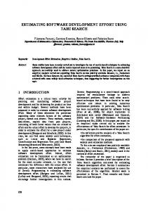
4. Effort distribution across phases As mentioned above the software process employed in the organization was waterfall-like, incorporating: • project planning (PP) • requirements specification (RS) • design specification and documentation (DES) • implementation (IMP) • test specification and testing (TEST) • release, installation and manuals (RIM) and • maintenance (MA). Effort records also accounted for training and learning (TL) and project management (PM). Distribution of effort for the sixteen projects shown by development phase is presented in Figure 1 and summarized over all activities in Table 1. It is evident from Figure 1 that records are most complete for the planning, design, implementation and testing phases. In many cases requirements specification effort (median 0.0%) was incorporated into planning or design, and release effort (median 0.9%) was included in the implementation and test effort records. A component of effort was also recorded as maintenance for nine of the sixteen projects (median 0.3%). It is clear from Table 1 that the bulk of project effort is taken up in the three phases of design, implementation and testing (median 76.9%), so it is on these phases that we focus our analysis. The histograms in Figure 1 also show that there is considerable variation in the distribution of phase effort among the sixteen projects – it does not appear that there is any sense of a ‘standard’ proportion of effort per phase. This is in contrast to the notion that we can accurately characterize the distribution of project effort using a typical breakdown [7, 32] (although we acknowledge that this outcome may not apply to all data sets). Note that for ease of viewing each histogram has a different scale yaxis. We therefore provide an alternative view of this data (for the core planning, design, implementation and test phases) in a single graph, shown in Figure 2. For this representation we have normalized the effort values for each phase to the scale 0 to 1, by dividing each observation by the maximum value per phase.

4

Proceedings of the Ninth International Software Metrics Symposium (METRICS’03) 1530-1435/03 $17.00 © 2003 IEEE

Figure 1. Distribution of effort per phase

Table 1. Summary of effort distribution per phase

Median Maximum Range Interquartile Range Outliers

PP 2.9% 13.9% 13.9% 4.1% 2

RS 0.0% 11.0% 11.0% 1.1% 1

DES 18.6% 37.7% 33.6% 15.0% 0

IMP 27.2% 77.3% 57.9% 20.2% 1

5

Proceedings of the Ninth International Software Metrics Symposium (METRICS’03) 1530-1435/03 $17.00 © 2003 IEEE

TEST 23.0% 44.0% 40.5% 12.2% 1

RIM 0.9% 7.1% 7.1% 2.2% 1

MA 0.3% 10.9% 10.9% 1.3% 1

TL 5.4% 27.2% 26.6% 6.8% 0

PM 7.7% 17.5% 13.9% 5.7% 0

1.000 Proportion PP of ACT (N)

0.900 0.800 0.700

Proportion DES of ACT (N)

0.600 0.500 0.400

Proportion IMP of ACT (N)

0.300 0.200

Proportion TEST of ACT (N)

0.100 0.000 1

3

5

7

9

11

13

15

Project

Figure 2. Normalized volatility of effort per phase Figure 2 enables us to get a sense of the relative use of labor in each phase for the sixteen projects in the data set. For instance, we can see that the extent of planning undertaken for projects 1 and 13 was relatively much greater than for the other fourteen projects. Design effort varies significantly from one project to another, with no discernible consistency or pattern over the projects. Normalized test effort exhibits several highs and lows (projects 6, 11 and 16, and projects 1, 7, 8 and 15, respectively) although the remaining nine projects exhibit slightly greater consistency, all falling between 0.40 and 0.59 on our normalized relative scale of 0 to 1. A more consistent pattern of relative effort appears to occur for the implementation phase, with ten of the normalized values falling between 0.25 and 0.36 and one clear outlier project (project 15). Overall, however, it appears that on the basis of the data set analyzed here, the distribution of effort over the life of a project varies substantially from one development to another, certainly until the bulk of effort has been expended. As a result we are not able to estimate the effort required for each phase using standard proportions. This leads us to consider whether useful significant relationships might exist among the proportions of effort required for project phases. For instance, a high proportion of effort in implementation might imply the need for a high proportion of testing effort; or, conversely, a larger proportion of effort expended in planning or requirements analysis may mean that a lesser proportion of effort is needed in later phases. We examined this issue by first transforming all sixteen projects to the same scale by multiplying all data values

so that total effort on the sixteen projects was the same, an approach that is appropriate given that here we were considering proportions rather than absolute values. We then examined the correlation values among the various proportions of effort, reported in Table 2. Significance at the 0.05 level is indicated by a single asterisk, a double asterisk (**) indicating significance to the 0.01 level. In this case we employed two-tailed tests, as we were unsure of the direction of any relationships that might be identified. Table 2 indicates that there are four significant relationships among the data for proportional effort per phase. The single positive relationship is that between planning and design effort, implying that as the proportion of planning effort changes so the proportion of design effort tends to change in the same direction. In contrast, increased planning effort implies reduced effort expended in implementation (as a proportion of total effort), as does increased design effort. These relationships can be seen graphically in Figure 3. (The significant relationship between requirements specification and testing should be treated with caution, as only eight of the sixteen projects had non-zero values for requirements specification effort.) These initial results suggest that there appears to be some potential benefit in investigating the relationships among effort expended over the various phases of a software project, although the precise nature of the relationships and their predictive capabilities is not known at this stage. In the absence of any standard proportions for effort in this data set we turn our attention to considering whether useful models might alternatively be produced using standard linear regression methods.

6

Proceedings of the Ninth International Software Metrics Symposium (METRICS’03) 1530-1435/03 $17.00 © 2003 IEEE

Table 2. Kendall’s tau correlation values for proportional effort per phase PP RS DES IMP TEST RIM MA

RS

.17** .50** -.42** -.15** -.17** -.05**

DES

.31** -.27** -.40** .09** -.08**

IMP

-.48** -.32** -.14** .03**

TEST

-.10** -.12** -.28**

RIM

.06** .36**

.12**

1 0.9 0.8 Proportion PP

0.7

Proportion

Proportion RS 0.6

Proportion DES

0.5

Proportion IMP Proportion TEST

0.4

Proportion RIM 0.3

Proportion MA

0.2 0.1 0 1

3

5

7

9

11

13

15

Project

Figure 3. Proportion of total development effort per phase

As a result we performed two-tailed correlation analysis using Kendall’s tau (reported in Table 4). Significance at the 0.05 level is indicated by a single asterisk, a double asterisk (**) indicating significance to the 0.01 level.

5. Model fitting The starting point for our regression-based modeling is bivariate correlation analysis. As stated in the previous section, our focus here is on the design, implementation and testing phases, as it is during these phases that effort requirements are greatest, and therefore where the need for accuracy is of most importance. We also include in our analysis the data on planning effort as this may be worth considering in terms of its relationship with design effort, and the records for planning are far more complete than those for requirements analysis. Descriptive statistics for these four variables are shown in Table 3. There is some evidence of asymmetry in the distributions of planning and test effort data, indicated by both the skewness values and the existence of outliers.

Table 3. Descriptive statistics – effort per phase

Mean 7

Proceedings of the Ninth International Software Metrics Symposium (METRICS’03) 1530-1435/03 $17.00 © 2003 IEEE

PP 103.4

DES 556.0

IMP 870.7

TEST 673.9

Standard Deviation Median Interquartile Range Skewness Outliers

119.7 64.0 104.4 1.8 2

474.4 398.0 806.0 0.8 0

620.1 844.0 970.4 0.5 0

2. use linear regression to construct four models a. univariate (effort for the prior phase) plus constant b. univariate (effort for the prior phase), no constant c. multivariate (effort for the prior phase and software category indicator) plus constant d. multivariate (effort for the prior phase and software category indicator), no constant 3. construct combined models a. for each observation take the arithmetic mean of the original estimate (OE) and the value estimated using the benchmark and linear regression models b. for each observation take the arithmetic mean of the current estimate (CE) and the value estimated using the benchmark and linear regression models 4. determine the sum of error and sum of absolute error of each model 5. compare the performance of each model to that achieved using expert estimates OE and CE.

772.1 328.0 1004.5 1.7 1

Table 4. Kendall’s tau correlation values for phase effort data

DES IMP TEST

PP 0.62** 0.25** 0.40**

DES 0.48** 0.58**

IMP

0.53**

On the basis of the correlation analysis it appeared that it might be possible to fit a number of models relating effort expended in earlier phases to that required in later stages of a project. The most straightforward approach would be to construct a model for each significant relationship, simply mapping one effort variable to another. However, this ignores the potential contribution of other variables in combination with the effort data, something that cannot be assessed using simple bivariate correlation analysis. We had two other potential predictor variables available in the data set – the intended operational environment, and the primary programming language to be used in development. Exploratory analysis of the potential contribution of phase effort with each of these two variables indicated that the likely software environment category would be useful in terms of fitting models of effort across phases. Further investigation revealed that in fact the two were very strongly related, in that in twelve of the sixteen projects the combination of intended environment and language was the same – software to be deployed in a non-runtime Unix environment was almost always developed primarily in C++, whereas runtime software was normally developed in C. As a result, we decided to use the four effort variables and the category indicator (a dummy variable, with value 0 for non-runtime software and value 1 for runtime) in the remainder of our analysis. Four relationships were therefore evaluated: design effort based on planning effort (DES), implementation effort based on design effort (IMP), testing effort based on design effort (TEST(D)), and testing effort based on implementation effort (TEST(I)). Our approach to model fitting for each relationship was as follows: 1. construct three benchmark models a. set all observations in the subsequent phase to zero b. use the average effort expended on projects to date to generate the next in sequence c. use the median effort expended on projects to date to generate the next in sequence

Tables 5 to 8 summarize the comparative performance of the expert, regression and combined expert/regression models where in every case the best regression or expert/regression model (that is, the model with the lowest error) is chosen. Values less than zero in the ‘OE/CE Sum of Error’ and ‘Model Sum of Error’ columns indicate that effort was overestimated in comparison to the actual values, whereas positive numbers indicate that effort was underestimated by the technique. A positive value in the ‘Difference’ column indicates that the chosen regression or combined expert/regression model is more accurate than the corresponding OE/CE ‘model’, whereas a negative value indicates that in general the expert estimates are closer to the actual effort records. The ‘Change in Error’ column shows the degree to which accuracy has improved (positive value) or deteriorated (negative value) relative to the expert model error, as a percentage. We also consider the change in error in relation to the amount of effort actually expended – if accuracy has improved through the use of regression modeling, is that improvement sufficiently large to warrant using such an approach? This is indicated as a percentage value in the ‘Gain/Loss’ column. The final item in each table is the number of individual observations that incur a lower error when determined using the model rather than the expert approach. The number of observations per phase is sixteen, meaning that the total number of ‘Improved Estimates’ possible across the three phases is 48. Note that in each table two sets of results are provided, reflecting the impact of a choice between using design or implementation effort in modeling test effort (i.e. TEST(D) or TEST(I)).

8

Proceedings of the Ninth International Software Metrics Symposium (METRICS’03) 1530-1435/03 $17.00 © 2003 IEEE

If an organization manages projects under a portfolio approach then their goal may be to simply minimize the sum of error – in other words, as long as overexpenditure of labor on one project task is compensated for by under-utilization on another, this is considered to be successful management of resources. Table 5 shows that at the beginning of the sixteen projects the managers underestimated implementation effort by 1982 personhours but overestimated testing effort by about the same amount (2234 person-hours). This could be interpreted as indicating an effort allocation problem – that is, the error was in the split of effort over the two phases (either estimated or recorded), rather than in the total amount of effort predicted. This is not supported, however, by the comments recorded by the managers, or in fact by the revised estimates (CE) produced later in the projects (see Table 7). Furthermore, whilst accuracy over an entire project is desirable, it is also important to have accurate phase estimates to enable effective management during projects. Given that the organization had recently revised their project management systems to enable more accurate records to be collected, it seems reasonable to consider the underlying data to be both correct and realistic. The original effort (OE) and revised effort (CE) figures therefore provide a useful benchmark against which to compare the alternative models. The models produced using prior-phase effort and the software category indicator resulted in error totals close to zero in all cases (see ‘Model Sum of Error’ in Table 5), an expected outcome given that regression models are built with the intention of minimizing error. Perhaps more useful is the fact that each of the models produced more accurate phase effort values than those provided by the project managers for a number of individual projects. It is interesting to note that the regression model that mapped design effort to testing effort (TEST (D)) was more accurate in nine of the sixteen cases whereas the model employing implementation effort as a predictor (TEST (I)) led to more accurate values in only four cases. Given that design records are available earlier in the process the first set of models would appear to be preferred in this case. Also worth noting is the comparatively low gain achieved in modeling design effort using planning effort – only a very slight reduction in error is achieved, and in fact the best regression model is outperformed by the project managers’ OE values for ten of the sixteen projects. Organizations that are concerned about the scale of error in estimation more than the direction of that error (through over- or underestimation) are likely to prefer to use the sum of the absolute error as a measure of overall accuracy. Assessment of the models against this criterion is shown in Table 6. Using this criterion the

original estimates were more than 17000 person-hours adrift of the effort that was actually expended over the three core phases of the sixteen projects. The alternative models produced by regression analysis improved this by a factor of more than one third (6040 person-hours), also resulting in more accurate values for 29 of the 48 observations. In this case the model that utilized implementation effort to determine testing effort proved to be more accurate than its design-based counterpart. It is clear from Table 6 that in general the gains in accuracy achieved through regression modeling are substantial, with that related to implementation effort being particularly strong at 30%. Design effort modeling is once more the exception, however, with a gain of just 1% in relation to total design effort. We now examine performance in relation to the managers’ revised effort estimates (CE) produced to reflect the impact of negotiated changes in software requirements. As these are normally produced as new information is gathered, it seems reasonable to expect that in general the current estimates (CE) would be more accurate than their OE predecessors. Taking the sixteen projects as a portfolio, however, we find that this is not the case (see Table 7). The revised estimates for design, implementation and testing effort resulted in a larger overall error than that achieved with the original estimates (2994 person-hours using CE vs -329 person-hours using OE). Testing effort accuracy was in fact improved in the revision process (by 469 person-hours), but this improvement was more than offset by substantially greater underestimation of design and implementation effort. As expected, regression-based models proved to be effective in minimizing overall error to close to zero, but in general this did not result in more accurate values for individual effort observations. In particular, just three of the sixteen design effort values were estimated more accurately using the alternative model even though overall error was reduced. In terms of the absolute error criterion (Table 8), the regression-based model for design effort performed worse than its CE counterpart, further bringing into question the advantage of regression modeling for this phase. This is in stark contrast to the improvements made in relation to implementation and testing, where the experts’ current estimates were significantly outperformed by the alternatives. The implementation model is particularly strong in that the selected model leads to a lower error for eleven of the sixteen project observations.

6. Discussion In the absence of standard effort proportions for development phases the object of the above analysis was

9

Proceedings of the Ninth International Software Metrics Symposium (METRICS’03) 1530-1435/03 $17.00 © 2003 IEEE

to determine whether it was feasible to improve on project managers’ estimates using prior-phase effort records.

10

Proceedings of the Ninth International Software Metrics Symposium (METRICS’03) 1530-1435/03 $17.00 © 2003 IEEE

-77 1982 -2234

DES IMP TEST (I) Total

1 4 -4

1 4 0

99% 100% 100%

99% 100% 100%

76 1978 2234 4288 76 1978 2230 4284

1% 14% 21% 13%

1% 14% 21% 13% 6/16 10/16 4/16 20/48

6/16 10/16 9/16 25/48

Difference Change in Gain/Loss Improved Estimates Error

3243 7888 6351

3243 7888 6351

DES IMP TEST (D) Total

DES IMP TEST (I) Total

3160 3688 4245

3160 3688 4594

OE Model Sum of Sum of Absolute Absolute Error Error 3% 53% 28%

3% 53% 33%

83 4200 1757 6040 83 4200 2106 6389

1% 30% 20% 19%

1% 30% 16% 18%

11

8/16 11/16 10/16 29/48

8/16 11/16 10/16 29/48

Difference Change in Gain/Loss Improved Estimates Error

Table 6. Minimizing sum of absolute error against OE

-77 1982 -2234

OE Model Sum of Sum of Error Error

Table 5. Minimizing sum of error against OE

DES IMP TEST (D) Total

Proceedings of the Ninth International Software Metrics Symposium (METRICS’03) 1530-1435/03 $17.00 © 2003 IEEE

986 3773 -1765

1 4 -4

1 4 0

100% 100% 100%

100% 100% 100%

985 3769 1765 6519 985 3769 1761 6515

11% 27% 16% 19%

11% 27% 16% 19%

2320 5651 5770

2320 5651 5770

DES IMP TEST (D) Total DES IMP TEST (I) Total

CE Sum of Absolute Error

2349 3688 3847

2349 3688 4268

Model Sum of Absolute Error

-1% 35% 26%

-1% 35% 33%

-29 1963 1502 3436 -29 1963 1923 3857

0% 14% 18% 11%

0% 14% 14% 10%

6/16 11/16 9/16 26/48

6/16 11/16 9/16 26/48

Difference Change in Gain/Loss Improved Estimates Error

3/16 9/16 4/16 16/48

3/16 9/16 8/16 20/48

Difference Change in Gain/Loss Improved Estimates Error

Table 8. Minimizing sum of absolute error against CE

DES IMP TEST (I) Total

CE Model Sum of Sum of Error Error DES 986 IMP 3773 TEST (D) -1765 Total

Table 7. Minimizing sum of error against CE

The model fitting analysis illustrates that (at least for our data set) there are potentially useful and consistent mappings from prior-phase effort data to that required in later phases. Retrospective fitting of regression and combined expert/regression models to the sixteen projects indicates that significantly better projections of effort could have been possible, enabling the organization to plan activities and allocate resources in a more cost-efficient way. Of interest is the extent to which the alternative (nonexpert) models contributed to reduction in error, either on their own or in combination with the expert estimates. In attempting to minimize the sum of error, multivariate regression models with a constant term proved to be the best (of the expert, benchmark, regression and combined expert/regression models) in all cases. When assessed using the sum of absolute error, the combined expert/regression approach proved to be the most accurate in the majority of cases. In only one instance – that of mapping planning effort to design effort – did the expert model using revised values (CE) outperform the alternative models. Overall then, these outcomes confirm that the use of more than one modeling method can provide some benefit in reducing overall error. Looking particularly at the data set analyzed here, it appears that modeling both implementation and testing effort on the basis of actual design effort could be especially beneficial, leading potentially to a reduction in error by thousands of person-hours over a project portfolio. In contrast, the relatively poor performance of the alternative models in determining design effort from planning effort suggests that there is little to be gained over expert estimation for this phase of development. But what of the general case? Artifact-based models – those based on product attributes such as the number of lines of code, the number of features, the number of function points and the like – have been used extensively in effort and schedule estimation. Questions remain, however, as to whether these approaches are sufficient to capture the factors that influence effort. Furthermore, the costs of data collection, analysis, training and so on associated with some of these methods can be non-trivial. While there is no doubt that there remains a real need for early effort predictions, which the approach advocated here cannot address, it may be that process-based models using actual effort and duration data could provide more accurate estimates as a project progresses. This analysis is not without its limitations. As this was a model-fitting exercise (to determine the feasibility of the approach) we used the complete data set to both determine the most useful models and to assess their potential worth in terms of improved estimates. As a result the analysis is optimistic and likely overstates the effectiveness of the approach. We were also constrained

in our analysis by only having access to the data – unfortunately because of demands on staff time we were not able to obtain detailed information on the projects and their progress. In particular, we were not able to ascertain the reasons for errors in estimation or unexpected progress outcomes. Such information would have enabled us to consider specific downstream effects – was the remainder of the schedule left as is? was functionality constrained in order to meet a fixed schedule? were effort and duration allocated for later phases adjusted? and if so, up or down, and by what amounts? That said, the magnitude of the improvements achieved using these very simple analysis methods justifies further investigation, even in the absence of project knowledge.

7. Conclusions In this paper we have described an empirical analysis based on the phase effort data derived from sixteen projects. There are three sets of findings: • There is little support for the idea of standard proportions of effort distributed between phases. Whilst this is only one study, it is potentially important, as it does not support the ideas of some software engineering researchers and commentators. • Our results verify that expert estimates can be improved upon through the use of models generated on the basis of prior-phase effort data. Importantly, these are models built using simple techniques and ideas that are accessible to busy professionals. • We provide further evidence to support the assertion that the use of more than one prediction technique can lead to more accurate estimates than if we rely on a single method. The next stage of this work is to consider the impact of the sequence in which projects are completed. In order to consider the usefulness of prior-phase effort models in a predictive setting we could use information on project completion to replicate the situation in which the data set grows over time as projects end. This would allow us to build predictive models that use only the records available at a given point in time to produce an estimate for the next project in the sequence. So to conclude, in terms of the wider significance of this research, the main observation to make is that yet again we have support for the value of local data, even when limited to only a few data points and relatively straightforward analysis methods.

Acknowledgements We are grateful to the company that provided the data

12

Proceedings of the Ninth International Software Metrics Symposium (METRICS’03) 1530-1435/03 $17.00 © 2003 IEEE

[17] G. Horgan, S. Khaddaj and P. Forte, "Construction of an FPAtype metric for early lifecycle estimation", Info. & Soft. Tech. 40, (1998): 409-415. [18] M. Höst and C. Wohlin, "A subjective effort estimation experiment", Info. & Soft. Tech. 39, (1997): 755-762. [19] R. Jeffery, M. Ruhe, and I. Wieczorek, “Using public domain metrics to estimate software development effort”, In Proc. 7th Intl Software Metrics Symposium. London, (2001): 16-27. [20] M. Jørgensen and D.I.K. Sjøberg, “Impact of effort estimates on software project work”, Info. & Soft. Tech. 43, (2001): 939948. [21] B. Kitchenham, "The certainty of uncertainty", In Proc. FESMA 98. The Netherlands (1998): 17-25. [22] A. Kulkarni, J.B. Greenspan, D.A. Kriegman, J.J. Logan and T.D. Roth, "A generic technique for developing a software sizing and effort estimation model", In Proc. COMPSAC '88. (1988): 155-161. [23] A.L. Lederer, R. Mirani, B.S. Neo, C. Pollard, J. Prasad and K. Ramamurthy, "Information system cost estimating: a management perspective", MIS Quart. (June 1990): 159-176. [24] H. Lee, "A structured methodology for software development effort prediction using the analytic hierarchy process", Jnl of Sys. & Soft. 21, (1993): 179-186. [25] W.E. Lehder, Jr., D.P. Smith and W.D. Yu, "Software estimation technology", AT&T Tech. Jnl, (1988): 10-18. [26] T. Lister, "Risk management is project management for adults", IEEE Software (May/Jun 1997): 20,22. [27] T. Lister, "Hallucinations at 37,000 feet", IEEE Software (May/Jun 1998): 105-107. [28] S.G. MacDonell and M.J. Shepperd, “Combining techniques to optimize effort predictions in software project management”, Jnl of Sys. & Soft. 66(2): 91-98. [29] S. McConnell, "Avoiding classic mistakes", IEEE Software (Sept 1996): 112, 111. [30] M.C. Ohlsson and C. Wohlin, "An empirical study of effort estimation during project execution", In Proc. 6th Intl Software Metrics Symposium. Boca Raton FL, (1999): 91-98. [31] A. Poulymenakou and A. Holmes, "A contingency framework for the investigation of information systems failure", Eur. Jnl Info. Sys. 5, (1996): 34-46. [32] L.H. Putnam and W. Myers Industrial Strength Software: Effective Management Using Measurement. Los Alamitos CA, IEEE Computer Society Press (1997) [33] A. Rainer and M. Shepperd, "Re-planning for a successful project schedule", In Proc. 6th Intl Software Metrics Symposium. Boca Raton FL, (1999): 72-81. [34] A.G. Rodrigues and T.M. Williams, "System dynamics in software project management: towards the development of a formal integrated framework", Eur. Jnl Info. Sys. 6, (1997): 5166. [35] I. Stamelos and L. Angelis, “Managing uncertainty in project portfolio cost estimation”, Info. & Soft. Tech. 43, (2001): 759768.

for this research. This work was undertaken while Dr MacDonell was a Visiting Researcher in the Empirical Software Engineering Research Group, School of Design, Engineering and Computing at Bournemouth University, with support from Auckland University of Technology and Bournemouth University. We are also grateful to the referees for their useful and constructive comments on the paper.

References [1] T.K. Abdel-Hamid, "On the utility of historical project statistics for cost and schedule estimation: results from a simulationbased case study", Jnl of Sys. & Soft. 13, (1990): 71-82. [2] T.K. Abdel-Hamid, "Adapting, correcting, and perfecting software estimates: a maintenance metaphor", Computer (Mar 1993): 20-29. [3] T.R. Adler, J.G. Leonard and R.K. Nordgren, "Improving risk management: moving from risk elimination to risk avoidance", Info. & Soft. Tech. 41, (1999): 29-34. [4] N. Ahituv, M. Zviran and C. Glezer, "Top management toolbox for managing corporate IT", Comm. ACM 42(4), (1999): 9399. [5] R. Baines, "Across disciplines: risk, design, method, process, and tools", IEEE Software (Jul/Aug 1998): 61-64. [6] R. Betteridge, "Successful experience of using function points to estimate project costs early in the life-cycle", Info. & Soft. Tech. 34(10), (1992): 655-658. [7] J.D. Blackburn, G.D. Scudder and L.N. Van Wassenhove, "Improving speed and productivity of software development: a global survey of software developers", IEEE Trans. Soft. Eng. 22(12), (1996): 875-885. [8] N. Brown, "Industrial-strength management strategies", IEEE Software (Jul 1996): 94-103. [9] M.J. Carr, "Risk management may not be for everyone", IEEE Software (May/Jun 1997): 21,24. [10] J. Charles, "CPM offers certificate in software estimating", IEEE Software (Nov 1996): 104-105. [11] B. Collier, T. DeMarco and P. Fearey, "A defined process for project postmortem review", IEEE Software (Jul 1996): 6572. [12] E.H. Conrow and P.S. Shishido, "Implementing risk management on software intensive projects", IEEE Software (May/Jun 1997): 83-89. [13] T. DeMarco Controlling Software Projects. New York NY, USA, Yourdon Inc. (1982) [14] R.L. Glass, "Software estimation is not a rational process", Jnl of Sys. & Soft. 23, (1993): 1-2. [15] R.L. Glass, "Short-term and long-term remedies for runaway projects", Comm. ACM 41(7), (1998): 13-15. [16] F.J. Heemstra, "Software cost estimation", Info. & Soft. Tech. 34(10), (1992): 627-639.

13

Proceedings of the Ninth International Software Metrics Symposium (METRICS’03) 1530-1435/03 $17.00 © 2003 IEEE