Using Public Domain Metrics to Estimate Software Development Effort Ross Jeffery University of New South Wales Centre for Advanced Empirical Software Research (CAESAR) Sydney, 2052, Australia
Melanie Ruhe University of Kaiserslautern Department of Computer Science 67663 Kaiserslautern, Germany
[email protected]
[email protected]
Abstract In this paper we investigate the accuracy of cost estimates when applying most commonly used modeling techniques to a large-scale industrial data set which is professionally maintained by the International Software Standards Benchmarking Group (ISBSG). The modeling techniques applied are ordinary least squares regression (OLS), Analogy-based estimation, stepwise ANOVA, CART, and robust regression. The questions we address in this study are related to important issues. The first is the appropriate selection of a technique in a given context. The second is the assessment of the feasibility of using multi-organizational data compared to the benefits from company-specific data collection. We compare company-specific models with models based on multi-company data. This is done by using the estimates derived for one company that contributed to the ISBSG data set and estimates from using carefully matched data from the rest of the ISBSG data. When using the ISBSG data set to derive estimates for the company generally poor results were obtained. Robust regression and OLS performed most accurately. When using the company’s own data as the basis for estimation, OLS, a CART-variant, and Analogy performed best. In contrast to previous studies, the estimation accuracy when using the company’s data is significantly higher than when using the rest of the ISBSG data set. Thus, from these results, the company that contributed to the ISBSG data set, would be better off when using its own data for cost estimation.
Isabella Wieczorek Fraunhofer Institute for Experimental Software Engineering (IESE) 67661 Kaiserslautern, Germany +49 6301 707 255
[email protected]
1. Introduction In recent years it has become possible to gain access to a large public domain data set available from the International Software Benchmarking Standards Group (ISBSG). This data set now contains data collected worldwide on 789 software projects. The data describes the nature of the projects and the organizations, the software developed, and the resources used on the project. The possibility thus exists for organizations to make use of this data set for benchmarking and as input to their cost estimation processes. However, little is known about the accuracy that might be expected when using this data for estimation or the most appropriate techniques to use in order to derive estimates or develop estimation models from the data. This study is motivated by the challenge of assessing the feasibility of using multi-organization data to build cost models for organizations and the benefits gained from company-specific data collection. The study looks at the prediction accuracy of different estimation techniques and examines their performance based on both multiorganizational and company-specific data sets. Thus, two important questions are addressed: (1) What are the differences in estimation accuracy between the different techniques? (2) Is there a difference between estimates derived from multi-company data and estimates derived from company-specific data? Recent publications have investigated some of these issues using earlier versions of the ISBSG data set [13], the Laturi and European Space Agency (ESA) [4, 5] data sets.
This is the first analysis of the ISBSG Release 6 data set for estimation. It is also the first study using data from an organization that has contributed to the data set and therefore used the data collection standards embodied in that data set. Thus, this paper reports on a continuing program of research to investigate the use of large datasets for estimation and the use of different methods of deriving estimation models and estimates from that data. The paper starts with a discussion of related work in Section 2 followed by the description of the data sets and the data preparation in Section 3. The design of this study, the estimation techniques, and the evaluation criteria are presented in Section 4. Section 5 describes the results of the analysis, and Section 6 and 7 present the conclusions and discussion of practical implications.
2. Related Work Little work has been published so far on the ISBSG database. Beside the work of the ISBSG group itself [12], a few studies have published their investigations on this data set in the areas of duration estimation [19], system sizing [15], and effort estimation [13]. Oligny and others [19] compared duration estimates obtained from simple COCOMO equations to an empirical model derived from the ISBSG data set (using Release 3 of the ISBSG dataset). Lokan [15] empirically investigated the validity of the Function Point measure (FP) analyzing relationships among the basic elements of this measure (using Release 4 of the dataset). The authors of this paper [13] compared two cost modeling techniques, namely Analogy and OLS regression, in terms of their accuracy using Release 5 of the dataset as well as another data set from an Australian company called Megatec. The comparative evaluation of cost modeling techniques has been the focus of many studies. Investigations have aimed to (1) determine which technique has the greatest effort prediction accuracy [4, 5, 10, 25, 27] and (2) propose new or combined techniques that could provide better estimates [6, 7, 9, 23, 31]. Due to the differences in the questions addressed, the techniques applied, the data sets used, and the designs applied for the comparisons, it is very difficult to draw generalizable conclusions from the results obtained at this stage of the research. Two other pieces of research have been completed which undertook a wide comparison of software cost modeling techniques. The first study [4] was based on the so-called “Laturi-database”, which included 206 business software projects from 26 companies in Finland. The
second study [5] was a replication of the first study using the European Space Agency (ESA) data set including 166 mainly space and military projects. In this research two questions were investigated. What modeling techniques are likely to yield more accurate results when using typical software development cost data? What are the benefits and drawbacks of using organization-specific data as compared to a multi-organization data set? Consistently, both studies found no significant advantages using local, company-specific data to build estimates over using external, multi-organizational databases. Moreover, in general Analogy-based techniques performed significantly worse than other traditional techniques such as OLS regression and stepwise Analysis of Variance. This paper explores the same questions and differs from these two earlier studies applying an additional modeling technique, namely robust regression. Little work has been reported so far on the application of robust regression for cost estimation purposes. Pickard, and others [20] investigated three techniques, namely residual analysis, multivariate regression and robust regression. The goal of this study was to evaluate these techniques using simulated data with different known characteristics. Miyazaki and others [16] tried to overcome the problems associated with OLS regression (results highly affected by outliers) and proposed a new robust method based on the least squares of inverted balanced relative errors. The evaluation was performed using five different data sets ranging from 10 to 48 projects from different applications. Another recent study by Gray and MacDonell [30] evaluated the accuracy of OLS regression, Artificial Neural Networks, and robust regression on three data sets known from the literature. The three studies give evidence that robust regression achieves promising accuracy levels. In line with the studies of Briand and others [4, 5], the current research contributes by evaluating many of the common modeling techniques using a large database. Moreover, we have included robust regression in our comparison, which has the potential to contribute to improved accuracy of the results. We apply a procedure consistent to our previous study [13], which was consistent with the comparative design applied in [4, 5]. This allows us to investigate (1) the feasibility of using multi-organizational data to build cost models and (2) the benefits gained from company-specific data collection. In the current case, the questions are investigated using an organization that contributed to the same database.
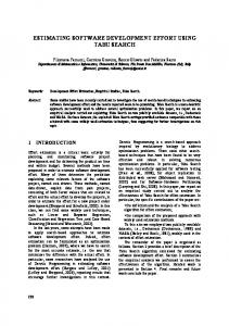
3. Data Set Description The database used in this study is the ISBSG repository (Release 6, December, 1999). The purpose of compiling the project database is to provide members with industrial output against which they may compare their projects, and to enable the analysis of delivery rates and the factors impacting upon delivery. The database contains 789 software projects collected worldwide in the time from 1990 to 1999. It is a mixture of new developments (53%), enhancements (41%), and re-developed projects (6%) that are characterized by many variables collected in conformance to international standards. The main contributing countries are Australia (31%), United States (22%), United Kingdom (12%), Canada (12%), France (9%), and the Netherlands (7%). The applications are mainly management information systems for a variety of business areas, such as banking, financial, manufacturing, legacy, or insurance. We selected variables that may potentially have an impact on project cost according to the following criteria: We only considered variables for which less than 40% of the data was missing. We did not consider variables that contribute to the calculation of an aggregated variable, such as the basic elements of the Function Point measure. If two or more variables contained redundant information, we only considered one of them, such as Function Points and Source Lines of Code (SLOC). Some variables include information about the quality of the data collected and the definitions of the type of data that was reported. We used these variables to further reduce the data set. The subset we used consisted of 325 projects with the highest assigned Quality Rating (Our goal here was to minimize the likely variance in the data arising from measurement error) and work effort data reported as data including development team effort (resource level 1) and support (resource level 2) (The goal here was to make the results as generalizable as possible by including measures of only project personnel rather than including user time, for example). In addition, one outlying observation was excluded from the data set. Thus, we ended up with 324 projects available for our analysis. Figure 1 depicts the stepwise reduction the of ISBSG data set for our analysis.
ISBSG Release 6 789 projects
Data Quality A 384 projects
Resource Level 1 & 2, 1 outlier excl.
Level 1 324 projects Level 2
Figure 1. Data set reduction of the ISBSG repository, release 6, for this study To then determine categorical variables that show a significant influence on productivity, we applied the nonparametric Kruskall-Wallis test [24]. For some of the variables, such as Organization Type, we merged the levels due to a very large number of levels and unbalanced proportions of observations per level. To do so, we used two criteria: (a) merge semantically similar levels, (b) if a level has less than 5 observations, and could not be merged according to (a), put under category “other”. The variables considered for our analysis are listed below. Effort is used as the dependent variable. Table 1. Variables used in this study Variable Name and definition Work Effort measured in person hours System Size measured in Function Points Maximum Team Size Development Platform Language Type Business Area Type Organization Type
Abbreviation used in the paper Effort FP MTS DevPlat LangType BAT OrgType
Furthermore, it was possible to identify the projects in the data set provided by one company. Table 2 presents the number of projects for each resource level and the number of projects for that company and for the rest of the selected data set. Table 2. Data sets used in this study Σ
12
ISBSG without one company 189
2
121
123
14
310
324
One company Resource Level 1 Resource Level 2 Σ
201
Table 3 summarizes descriptive statistics for ratioscaled variables for the one company as well as for the reduced multi-company data set of 324 projects. The project delivery rate (PDR) is used as a measure of
productivity. This measure is used in line with the ISBSG [12]. It is defined as working hours per Function Point. A high number indicates that many hours per Function Point were needed and, therefore, indicates a low productivity and vice versa. Table 3. Project Characteristics for the ratio-scaled variables One Company FP Effort MTS PDR
256 560 2.8 2.2
ISBSG FP Effort MTS PDR
median 267 568 2 2.0
min
max
56 170 1 1.4
579 1238 8 3.8
324 projects 633 4780 6.0 9.5
259 1936 4.0 7.0
9 97 1 0.4
17518 59809 55 73.5
Table 3 shows large differences between companyspecific projects and ISBSG projects in terms of mean Function Points, mean effort, mean team size, and especially mean PDR. On average, projects from the one company are much more productive (evidenced in lower PDR values) compared to the whole ISBSG database. Also, the variables’ variance is much larger for the whole database compared to the company-specific projects. Table 4 summarizes the mean PDR and mean effort values for some of the nominal dependent variables. The values for the variables Business Area Type and Organization Types are presented in the Appendix. Table 4. Project Characteristics for some of the nominal variables One Company Resource Level DevPlat LangType
14 projects Mean Mean effort PDR 1 2 PC MR 4GL
ISBSG Resource Level DevPlat
LangType
615 232 534 893 560
2 2 2 3 2
324 projects 1 2 PC MR MF ApG 2GL 3GL 4GL
4. Research Method This section briefly describes the concepts and actual settings of the techniques applied, the criteria used to evaluate the accuracy, and the design of the study.
4.1. Modeling Techniques Applied
14 projects mean
Again, the large difference between the company and the multi-company data is evidenced.
4929 4537 2492 5408 5216 7981 3504 5596 3629
8 12 7 11 7 8 3 12 7
We considered the set of techniques that have been proposed in previous studies. These techniques were selected according to high-level criteria that are important from a practical perspective. These are techniques for which the models are interpretable, which can be automated, and for which at least an initial utility has been demonstrated in software engineering. The modeling techniques that fulfilled those criteria are: Ordinary Least Squares Regression (OLS) [22], stepwise Analysis of Variance (stepwise ANOVA) [14], Regression Trees (CART) [3], and Analogy [27]. In addition, we applied robust regression [21] techniques, which have been rarely applied so far for cost estimation purposes. OLS Regression OLS is the most common modeling technique applied to software cost estimation [8]. It fits the data to a specified model trying to minimize the overall sum of squared errors. There are several common concepts and assumptions when applying the technique. We refer to [11] for further details. We applied multivariate regression analysis fitting the data to an exponential model specification. We performed logarithmic transformations of the ratio-scaled variables and generated dummy variables [22] for the nominal scaled variables. A mixed stepwise procedure was applied (probability to enter/leave the model=0.05) to determine variables having a significant impact on effort. Stepwise ANOVA Stepwise ANOVA combines a variety of techniques to analyze the variance of unbalanced data [14]. It applies ANOVA to categorical variables and OLS regression to continuous variables. The stepwise procedure includes one (the most significant) independent variable at a time into a linear model. Its effect is removed transforming the dependent variable into a residual variable. Then the impact of each remaining independent variable on the residual is assessed to identify the next variable to include in the model. The analysis is repeated until all significant variables are found.
We transformed the continuous variables applying their natural logarithms. This was done to ensure normally distributed dependent variables. Consistent with previous studies [4, 5], we used effort as the dependent variable (techniques referred to as ANOVA_e). In addition, we used productivity (PDR) as a dependent variable, which is in line with [14] (referred to as ANOVA_p). In the case where PDR was a dependent variable the set of independent variables was reduced to exclude the variable system size (FP). CART The CART algorithm builds a model in form of a tree by recursively splitting the data set until a stopping criterion is satisfied [3]. The best split is the one that most successfully separates the high from the low values of the dependent variable [20]. All but the terminal nodes in a tree specify conditions. A project can be classified by starting at the root node of the tree and selecting a branch to follow based on the project’s specific variable values. One moves down the tree until a terminal node is reached. Consistent with several studies [4, 5, 14], we used productivity as a dependent variable (referred to as CART_p). Additionally, we used effort as a dependent variable consistent with [25] (referred to as CART_e). The stopping criterion was set to a minimum of 10 observations in each terminal node. Predictions were based on the median value of the dependent variable and we used the LAD (least absolute deviation) as the splitting criterion. Analogy-based estimation The potential of Analogy-based estimation for software cost estimation has been evaluated and confirmed in many studies [2, 18, 23, 27]. Analogy is a common problem solving technique. In software effort estimation, Analogybased estimation involves the comparison of a new (target) project with completed (source) projects. The basic idea is to identify source projects that are most similar to the new project. Major issues are (1) to select relevant project attributes (in our case cost-drivers), (2) to define an appropriate similarity function, and (3) to decide upon the number of similar source projects to consider for estimation (analogues). Some strategies exist to determine relevant project attributes [10, 23]. We used the variables from Table 1 as they had a significant impact on productivity (PDR). This approach is in line with Finnie’s strategy [10]. Similarity functions may be defined with the help of experts. We applied a simple measure proposed by
Shepperd in the ANGEL tool: the unweighted Euclidean distance using variables normalized between 0 and 1 [29]. For effort prediction, one may consider one or more source projects. This decision is made on a case-by-case basis since no heuristic currently exists. However, some studies report no significant differences in accuracy when using different numbers of analogues [4, 23]. Another recent study [1] concluded that the best choice for the number of analogies was one project. The study showed that an increase of the number of analogs causes an increase in MMRE. This was demonstrated by creating empirical distributions of MMRE values for an increasing number of analogies using a particular data set. For the sake of simplicity and based on the results of these studies, our predictions were based on the most similar project. We applied three different variants of Analogy-based on the suggestions by [4, 23, 27]. In this paper, we only present the best results obtained. We used the Euclidean distance as a measure for determining analogous projects (in consistency with [4] and [23]). Additionally, we applied linear size adjustment as suggested by [27]. The linear size adjustment addresses the differences in size between target (estimated) and source (most similar) project. The equation below defines how the predicted effort was adjusted. FP Effort ESTIMATED = ESTIMATED × EffortSOURCE FPSOURCE Robust Regression Robust regression aims to overcome the disadvantages of OLS regression minimizing the impact of outliers. We used an iterative robust procedure implemented in the STATA tool [26]. The basic ideas are described in [21]. As the ISBSG data is a rather unbalanced data set, robust regression was chosen [14]. Robust regression iteratively performs weighted OLS regressions. It calculates weights based on absolute residuals, and regresses again using those weights. Thus, outlying observations are given lower weights than normal observations. The iteration stops when the maximum change in weights drops below a certain tolerance. The weights are derived from a combination of two weight functions. (Huber’s function and bi-weights). Both weighting functions are used because Huber weights have problems dealing with severe outliers, while bi-weights sometimes fail to converge or have multiple solutions. As independent variables we used the ones identified as significant in the applied stepwise OLS regression procedure.
Table 5 lists the techniques applied in the current study and the acronyms used within the paper.
4.3. Study Design
Table 5. Techniques applied an their abbreviations
If one constructs a cost estimation model using a particular data set, and then computes the accuracy of the model using the same data set, the accuracy evaluation will be optimistic [28]. The cross-validation approach we use involves dividing the whole data set into multiple train and test sets, calculating the accuracy for each test set, and then aggregating the accuracy across all the test sets. To determine the accuracy of deriving local cost estimation models we used 14 projects coming from the one company. We applied a 14-fold cross validation approach. For each of the 14 projects from the one company, we used the remaining 13 as a basis for model building. The overall accuracy was aggregated. Calculating accuracy in this manner indicates the accuracy to be expected if an organization built a model using its own data set, and then uses that model to predict the cost of new projects. In order to determine the accuracy of estimates based on multi-organizational data, we partitioned the rest of ISBSG (310 observations) into two partitions according to the resource levels. This is justified, as significant differences in terms of PDR between those two resource levels were observed. The first partition consisted of 189 projects that collected working effort based on resource level 1 (development team effort). The second partition consisted of 121 projects that reported working effort according to resource level 2 (development team effort and support). The prediction based on multi-company data was done for each resource level separately. Thus, to predict the effort for the one company, we used resource level 1 projects external to the company (first partition) to predict the corresponding 12 projects from the company. Accordingly, we used resource level 2 projects external to the company (second partition), to predict the 2 projects from the company (see also Table 1).
Technique OLS Regression Stepwise ANOVA with effort as dependent variable Stepwise ANOVA with PDR as dependent variable CART with effort as dependent variable CART with PDR as dependent variable Analogy-based estimation Robust Regression
Abbreviation OLS ANOVA_e ANOVA_p CART_e CART_p Analogy RobReg
4.2. Evaluation Criteria The evaluation of the cost estimation models was done by using the following common criteria [9]. The magnitude of relative error as a percentage of the actual effort for a project, is defined as: Effort ACTUAL − Effort ESTIMATED MRE = Effort ACTUAL The MRE is calculated for each project in the data sets. Either the mean MRE or the median MRE aggregates the multiple observations. The median MRE is less sensitive to extreme values. A mean MRE of 0.50 means that on average the estimates are within 50% of the actual values. In addition, we used the measure prediction level Pred. This measure is often used in the literature and is a proportion of a given level of accuracy: Pred( l ) =
k N
Where, N is the total number of observations, and k the number of observations with an MRE less than or equal to l. A common value for l is 0.25, which is used for this study as well. The Pred(0.25) gives the percentage of projects that were predicted with an MRE equal or less than 0.25. Conte et al. [9] suggest an acceptable threshold value for the mean MRE to be less than 0.25 and for Pred(0.25) greater or than 0.75. In general, the accuracy of an estimation technique is proportional to the Pred(0.25) and inversely proportional to the MRE and the mean MRE. For testing the statistical significance between paired samples we used the Wilcoxon matched pairs test, a nonparametric analogue to the t-test [24].
5. Results The following Section presents the results of applying the estimation techniques on the data set. Section 5.1 and Section 5.2 report on evaluating the accuracy of estimation techniques. This addresses our first question stated in Section 1. Section 5.3 compares company-based estimates to ISBSG-based predictions. This addresses the second question stated in Section 1. Section 5.4 provides the results obtained from a calibration of ISBSG-based estimates. It is important to note that not all estimation techniques applied here were able to provide predictions
when there was missing data for a project. For example, OLS regression cannot cope with missing data related to the parameters used in their specifications. To ensure a valid comparison of all the applied techniques, we selected a subset of projects from our holdout sample of 14 projects for which there was no missing data. In our case all techniques were able to provide 12 predictions for the one company. Therefore, the results presented below are based on 12 predicted data points.
2.4
2.0
1.6
1.2
0.8
0.4
5.1. Results based on company-specific data 0.0
In the first step of our analysis, we derived effort estimates for the one company by using its own projects for model building. Table 6 shows the aggregated results in terms of mean and median MRE values, Pred (0.25), and R2 values. Figure 4 shows box plots of the MRE values for each of the techniques applied. Table 6. Prediction accuracy for estimates based on company-specific data applied on the company Estimation Method Analogy OLS Robust Regression ANOVA_p ANOVA_e CART_p CART_e
Mean MRE 0.305 0.254 0.320 0.489 0.297 0.238 0.760
Median MRE 0.208 0.228 0.263 0.475 0.276 0.178 0.451
Pred (0.25) 0.58 0.58 0.50 0.00 0.42 0.67 0.25
R2 0.42 0.47 0.32 0.48 0.36 0.46 0.69
It is noticeable that ANOVA_p and CART_e obtain higher mean and median MRE values than the other techniques. Also, the application of Analogy, OLS, robust regression, and CART_p obtains Pred(0.25)-values of at least 50%. Analogy and CART_e show a large variation in MRE values, which is caused by outlying predictions. CART_e predicts with very large errors for 3 projects. The relatively poor performance of CART_e in comparison to CART_p might be explained by the homogenous distribution of the product delivery rate (PDR) whereas effort is quite different for each project.
ANALOGY
ROBREG OLS
ANOVA_E ANOVA_P
CART_E CART_P
Non-Outlier Max Non-Outlier Min 75% 25% Median Outliers
Figure 3: Box plots of the MRE values for company based estimates To determine statistically significant differences among the techniques, we applied the Wilcoxon matched pair test [24]. Table 10 presents the p-values. The gray shading indicates a significant difference. Table 7: Comparison of the techniques when using the company’s own data (Wilcoxon test results) Estimates based on company-specific projects Ana OLS Rob Anova logy Reg _p 0.695 OLS 0.022 0.814 RobReg 0.017 0.059 0.099 Anova_p 0.754 0.814 0.583 0.071 Anova_e 0.007 0.754 0.638 0.388 CART_p 0.041 0.084 0.136 0.754 CART_e
Anova _e
CART _p
0.028 0.034
0.023
Taking into account these results we suggest the following ranking of the techniques in terms of accuracy: 1. 2. 3.
Analogy, OLS, and CART_p Robust regression and ANOVA_e ANOVA_p and CART_e
(1) Analogy, OLS, and CART_p do not show significantly different results and are not outperformed by any other technique. On the other hand, each of them outperform at least one technique significantly. (2) ANOVA_e and robust regression performs significantly better than one technique (i.e., CART_e, ANOVA_p) and significantly worse than another technique (i.e., CART_p, OLS). (3) ANOVA_p and CART_e perform the worst. Both do not significantly outperform any other technique and at least two other techniques significantly outperformed ANOVA_p or CART_e.
Table 9. Comparison of the techniques when using multi-company data (Wilcoxon test results)
5.2. Results based on ISBSG-based data As a second step in our analysis, we derived effort predictions the one company using carefully matched ISBSG projects for model building. This was done with the reduced data and separately for each resource level as explained in Section 4. The aggregated accuracy results are presented in Table 8. depicts the ranges of MRE’s for each technique applied. Table 8. Prediction accuracy for ISBSG based estimates applied to one company Estimation Method Analogy OLS Robust Regression ANOVA_p ANOVA_e CART_p CART_e
Mean MRE 1.145 0.895 0.848 1.234 1.304 1.935 1.563
Median MRE 0.701 0.683 0.638 1.124 1.137 2.129 1.316
Pred (0.25) 0.17 0.00 0.00 0.00 0.00 0.08 0.08
R2 0.36 0.50 0.52 0.66 0.73 0.38 0.73
In general, the prediction accuracy is very low (high mean and median MRE values, low Pred(0.25) values). Analogy, OLS, and robust regression performed slightly better than the other techniques. Both ANOVA and CART perform similarly poor. 5
4
Estimates based on multi-company projects Anova Ana OLS Rob _p logy Reg 0.347 OLS 0.034 0.099 RobReg 0.012 0.004 0.875 Anova_p 0.002 0.003 0.347 0.638 Anova_e 0.034 0.008 0.009 0.023 CART_p 0.028 0.638 0.388 0.084 CART_e
Anova _e
CART _p
0.034 0.937
0.182
The results from above suggest the following accuracy ranking of techniques when using multi-company data for predicting effort: 1. Robust Regression 2. Analogy and OLS 3. ANOVA_e and ANOVA_p 4. CART_e and CART_p (1) The Wilcoxon test confirms that both OLS and robust regression perform best. (2) Surprisingly, there is also a significant difference between OLS and robust regression (0.034). It seems that robust regression is slightly better than OLS regression when looking at Table 8. Analogy does not show significant differences to any other technique than CART_p. (3) There is no difference among the ANOVA variants which are significantly outperformed by two other techniques. (4) Furthermore, both CART variants have practically no different results. Also, many other techniques outperform CART_p, whereas one technique outperforms CART_e.
3
5.3. Comparison of company-based versus ISBSG-based predictions
2
1
0
ANALOGY2 OLS
ROBREG ANOVA_E CART_E ANOVA_P CART_P
Non-Outlier Max Non-Outlier Min 75% 25% Median Outliers
Figure 4. Box plots of the MRE values for ISBSG based estimates OLS and Robust regression show a lower variation in their MRE values compared to the other techniques. CART_e and CART_p perform with widely ranged MRE’s. To test for the significance in the accuracy differences among the selected techniques we again applied the Wilcoxon matched pairs test. The p-values in Table 9 are used to identify a ranking of the estimation techniques.
To investigate the differences between estimates derived from ISBSG-based data and estimates derived from company-specific data we again we applied the Wilcoxon matched pairs test. For each modeling technique the accuracy of these two types of estimates was compared.
Table 10. Company-based versus ISBSG-based estimates: p-values from Wilcoxon test Comparison
Median MRE for company based estimates 0.208 0.228 0.263 0.475 0.276 0.178 0.451
Analogy OLS Robust Reg. ANOVA_p ANOVA_e CART_p CART_e
Median MRE for ISBSG based estimates
p-value
vs
vs vs vs vs vs vs vs
0.701 0.683 0.638 1.234 1.137 2.129 1.316
0.023 0.004 0.018 0.005 0.002 0.003 0.136
Table 10 shows significant differences for all but one technique. Comparing also Table 6 with Table 8 it seems obvious that company-based predictions are much more accurate than the predictions based on the ISBSGprojects.
5.4. Calibration of multi-company-based estimates The main reasons for the poor predictions based on the multi-company data are the large differences in productivity and effort (see Figure 4 and Table 3, Table 4) for the company compared to the rest of the ISBSG data. The mean PDR of the ISBSG projects excluding the company is about 5 times higher than the mean PDR of the company. Level1 & 2 without company 200 175
difficult to accurately predict effort for this particular company using the rest of the ISBSG data. In order to address the differences between the company and the ISBSG in general, we adjusted the predictions by the ratio of the mean PDR values. The following formula was used: (see also [17]).
Effort Adjusted =
meanPDRcompany meanPDRISBSG
× Effortpredicted
This assumes, of course, that a company has already collected a substantial amount of data from past software projects and is able to determine an average productivity rate or that it can be estimated in some other way. Table 11. Prediction accuracy for ISBSG based estimates with productivity adjustment Estimation Method Analogy OLS Robust Regression ANOVA_p ANOVA_e CART_p CART_e
Mean MRE 0.54 0.61 0.62 0.48 0.46 0.36 0.49
Median MRE 0.65 0.60 0.61 0.50 0.49 0.26 0.45
Pred (0.25) 0.17 0.00 0.00 0.08 0.17 0.50 0.08
Table 11 presents the results after applying the productivity adjustment. Compared to the results in Table 8 ANOVA and CART perform much better than without productivity adjustment. Analogy and OLS however, do not show large improvement. The biggest improvement was obtained for CART_p.
150
No of obs
125
1.0
100 75
0.8
50 25 0
0
10
20
30
40
50
60
70
80
0.6
PDR
No of obs
Company 4 2 0
0.4 0
1
2
3
4
5
PDR
0.2
Figure 5. Histograms of the PDR Having a closer look at the predictions based on multicompany data, we found general over-estimations for 7 of the 12 target projects. In addition, when applying ANOVA or CART all of the predictions were too high. Although, we tried to reduce the variance in the data itself as explained in Section 3 it seems to be quite
0.0
ANALOGY
ROBREG OLS
ANOVA_E ANOVA_P
CART_E CART_P
Non-Outlier Max Non-Outlier Min 75% 25% Median Outliers
Figure 6. Box plots of the MRE values for ISBSG based estimates with productivity adjustment
The results are confirmed in the box plots. Furthermore, the range of MRE values generally decreased (compare to Figure 4).
6. Discussion The particular aims of this study were twofold. Firstly, we investigated the differences in estimation accuracy between the different modeling and estimation techniques, and secondly, we compared estimation accuracy using multi-company data as input compared with companyspecific data. For the first of these techniques we have applied robust regression to a large industrial software engineering dataset for the first time. The results are indeed encouraging. This technique generally minimizes the mean and median MRE for both input data sets. It also has the advantage of being a relatively straightforward technique to apply in comparison with say CART and ANOVA which is an important consideration in industrial settings without specific tool support. Another promising result is the relative success of OLS and Analogy used here. The industrial benefits of Analogy are presented in [27] and OLS also is a well-understood technique. It also seems that the contrasting result for Analogy in this study with those of Briand and others [4, 5] indicates a need to further develop our understanding of analogical selection and prediction. The relative inaccuracy of CART and ANOVA when using the rest of the ISBSG as input also deserves further investigation, particularly if other data sets can be located. For the second research question (data input) it is clear that the one company identified is significantly different to the average ISBSG organization. The effort patterns seen in their data are relatively predictable using the stored variables, as evidenced by lower MRE values in comparison with prior studies of this type. A best value median MRE of 18% (mean MRE 24%) clearly indicates the viability of data-driven estimation using relatively simple models and modeling techniques. The picture is not as clear however concerning their use of the ISBSG dataset. Without productivity adjustment the MRE values are unacceptably high and much higher than seen in the prior study of the ISBSG data [13]. These results indicate, not surprisingly, that the variance in the data attributable to unidentified organizational processes as opposed to the identified characteristics of the software, hardware, system or organization type can be high. This then reveals that these data sets should contain an organizational I.D. at least so that this factor can be used in modeling. Further
progress in understanding the dynamics will not really be possible until process measures (such as SPICE or CMM) are linked to these benchmarking datasets. As more studies of this type are completed it becomes possible to begin building a picture of the usefulness of cost estimation techniques and industry data sets for cost estimation. The earlier studies based on the “Laturi” [4] and ESA data [5] found that (1) standard techniques such as OLS or ANOVA performed as well as or better than the other modeling and estimation techniques applied. In this study only OLS performed relatively well. (2) there were no accuracy benefits in using companyspecific data over external multi-organizational data. This result was not confirmed in this study. In the first study of the ISBSG data [13] it was found that that OLS regression performed as well as Analogybased estimation when using company-specific data for model building. It was suggested that this was because of the understanding of the company’s cost drivers that could be embodied in the ranking and selection rules of Analogy. Using multi-company data the OLS regression model provided significantly more accurate results than Analogy-based predictions. Furthermore, predictions based on company-specific projects data were significantly more accurate than predictions based on external data.
7. Conclusions The company studied here is a software company developing systems for a single organization. Because of confidentiality requirements associated with the ISBSG we have no further knowledge of the companies involved or their software development maturity. In this study we have found that the one company would be ill advised to use the ISBSG data set for estimation but that they could achieve relatively accurate estimates using their own data. The broader question addressed concerning techniques indicates that robust regression is a contender and OLS and Analogy continue to perform well. When we put the series of results together from the various studies, there are still a number of unanswered questions. Without data of their own, how can an organization determine if the multi-company dataset will be descriptive of their type of operation? If a company has its own data is the multi-company data of added value in estimation (as opposed to benchmarking). Given the conflicting results for Analogy, what is the best analogical
approach? Will the positive results for robust regression be confirmed in other datasets? Will further measurement of process and product variables improve the estimation accuracy derived from multi-company datasets? In this study we have been able to add to our knowledge of modeling and estimation techniques and the questions of estimation accuracy. The robust regression results need replication however, and the issue of how an organization can confidently decide on the use of public datasets in estimation needs further investigation. That an organization will need to identify firstly whether they are “like” organizations in the public data set is clear. We have shown that the one company has a higher productivity than average. The gross productivity adjustment applied is a blunt instrument that makes general improvement in the estimation accuracy. It is now important that the data sets move beyond simple productivity benchmarking so that process/product relationships can be better understood and applied.
8. References
Assessment. In: Proceedings of the 20th International Conference on Software Engineering, ICSE 98, pp. 390-399. [8] L.C. Briand, I. Wieczorek. Software Resource Estimation in Software Engineering. Accepted for Publication in: Encyclopedia of Software Engineering. John Wiley & Sons. [9] S.D. Conte, H.E. Dunsmore, V. Y. Shen. Software engineering metrics and models. The Benjamin/Cummings Publishing Company, Inc., 1986. [10] G.R. Finnie, G.E. Wittig. A comparison of software effort estimation techniques: using function points with neural networks, case based reasoning and regression models. J. Systems Software, 39 (1997), pp. 281-289. [11] W. Hayes. Statistics. Fifth Edition. Hartcourt Brace College Publishers. 1994 [12] Software Project Estimation: A Workbook for MacroEstimation of Software Development Effort and Duration, ISBSG, 1999.
[1] L. Angelis, I. Stamelos. A Simulation Tool for Efficient Analogy Based Cost Estimation, Empirical Software Engineering, 5, pp. 35-68, (2000)
[13] R. Jeffery, M. Ruhe, I. Wieczorek. A Comparative Study of Two Software Development Cost Modeling Techniques using Multi-organizational and Company-specific Data. In: Proceedings of the ESCOM 2000, Munich, 2000, pp. 239-247
[2] R. Bisio, F. Malabocchia. Cost Estimation of Software Projects through Case Based Reasoning. Case Based Reasoning Research and Development, In: Proceedings of the International Conference on Case-Based Reasoning, pp. 11-22, (1995)
[14] B. Kitchenham. A. Procedure for Analyzing Unbalanced Data Sets, IEEE Transactions on Software Engineering, 24, 4 (April 1998), pp. 278-301.
[3] L. Breiman, J.H. Friedman, R.A. Olshen, C.J. Stone. Classification and Regression Trees. Wadsworth & Books/Cole Advanced Books & Software (1984).
[15] C. Lokan. An Empirical Study of the Correlations Between Function Point Elements. In: Proceedings of the 6th International METRICS Symposium, November 1999, 200-206.
[4] L.C. Briand, K. El Emam, K. Maxwell, D. Surmann, I. Wieczorek. An Assessment and Comparison of Common Software Cost Estimation Models. In: Proceedings of the 21st International Conference on Software Engineering, ICSE 99, Los Angeles, USA 1999, pp. 313-322.
[16] Y. Miyazaki, M. Terakado, K. Ozaki, H. Nozaki. Robust Regression for Developing Software Estimation Models. J. Systems Software, 1994, pp. 3-16.
[5] L.C. Briand, T. Langley, I. Wieczorek. A replicated Assessment of Common Software Cost Estimation Techniques. In: Proceedings of the 22nd International Conference on Software Engineering, ICSE 2000, Limerick, 2000, pp. 377386. [6] L.C. Briand, V. R. Basili, W. M. Thomas. A pattern recognition approach for software engineering data analysis. IEEE Transactions on Software Engineering, 18, 11 (1992), pp. 931-942. [7] L.C. Briand, K. El Emam, F. Bomarius. A Hybrid Method for Software Cost Estimation, Benchmarking, and Risk
[17] Y. Miyazaki, K. More. COCOMO evaluation and tailoring. In: Proceedings of the 8th Conference on Software Engineering, 1985 [18] T. Mukhopadhyay, Vicinanza, S.S., Prietula, M.J. Examining the feasibility of a case-based reasoning model for software effort estimation. MIS Quarterly, pp. 155-171, (June 1992) [19] S. Oligny, P. Bourque, A. Abran. An Empirical Assessment of Project Duration in Software Engineering. In: Proceedings of the ESCOM 1997, Berlin, 1997. [20] L. Pickard, B. Kitchenham, S. Linkman. An Investigation
of Analysis Techniques for Software Data Sets. In: Proceedings of the METRICS 99 Symposium, Boca Raton, 1999, pp. 130141. [21] P.J. Rousseeuw; A.M. Leroy. Robust Regression and Outlier Detection, John Wiley & Sons, 1987. [22] L. Schroeder, D. Sjoquist, P. Stephan. Understanding Regression Analysis: An Introductory Guide. No. 57 In Series: Quantitative Applications in the Social Sciences, Sage Publications, Newbury Park CA, USA, (1986) [23] M. Shepperd, C. Schofield. Estimating software project effort using analogies. IEEE Transactions on Software Engineering, 23, 12 (November 1997), pp. 736-743. [24] D. Sheskin. Handbook of Parametric and Non-parametric Procedures. CRC Press. 1997 [25] K. Srinivasan, D. Fisher. Machine learning approaches to estimating software development effort. IEEE Transactions on Software Engineering, 21, 2 (February 1995), pp. 126-137. [26] StataCorp, Stata Statistical Software: Release 5.0. Stata Corporation, College Station, (Texas 1997). [27] F. Walkerden, R. Jeffery. An Empirical Study of Analogybased Software Effort Estimation. Empirical Software Engineering, 42, June 1999, pp. 135-158. [28] S. Weiss, C. Kulikowski. Computer Systems that Learn. Morgan Kaufmann Publishers, Inc. San Francisco, CA, (1991). [29]. [30] A. Gray, S. MacDonell. Software Metrics Data Analysis – Exploring the Relative Performance of Some Commonly Used Modeling Techniques. Empirical Software Engineering, 4, 1999, pp. 297-316. [31] E. Stensrud, I. Myrtveit. Human Performance Estimation with Analogy and Regression Models. In: Proceedings of the METRICS 98 Symposium, (1998) 205-213.
Appendix Table 12. Table of the categories of the nominal variable business area type (324 projects) Category Accounting & Legal Banking Engineering Financial (excluding Banking) Insurance Inventory Manufacturing Personnel Sales Telecommunications Other
Mean effort 7816 4828 1494 6402 4166 5135 5377 8593 1804 861 4022
Mean PDR 7.1 12.9 8.3 8.1 13.4 8.2 7.1 8.7 9.9 4.9 6.7
Table 13. Table of the categories of the nominal variable organization type (324 projects) Category Aerospace / Automotive Banking Chemicals Communication & Other Electricity, Gas, Water & Energy Financial, Property & Business Services Insurance Manufacturing & Other Public Administration Wholesale & Retail Trade Other
Mean effort 6834 4644 1174 6494 1682
Mean PDR 5.9 15.9 7.0 8.3 4.2
4483
9.7
3830 4859 4231 4887 7305
13.8 7.3 8.6 3.3 7.3