Using Quantile Regression to Estimate Capital Buffer Requirements ...

Using Quantile Regression to Estimate Capital Buffer Requirements for Japanese Banks

David E. Allen School of Accounting, Finance and Economics, Edith Cowan University, Australia Robert Powell1 School of Accounting, Finance and Economics, Edith Cowan University, Australia Abhay Kumar Singh School of Accounting, Finance and Economics, Edith Cowan University, Australia

Abstract This paper investigates the impact of extreme fluctuations in bank asset values on the capital adequacy and default probabilities (PD) of Japanese Banks. We apply quantile regression analysis to the Merton structural credit model to measure how capital adequacy and PDs fluctuate over a 10 year period incorporating the Global Financial Crisis (GFC). Quantile regressions allow modelling of the extreme quantiles of a distribution, as opposed to focussing on the mean, which allows measurement of capital and PDs at the most extreme points of an economic downturn. Understanding extreme risk is essential, as it is during these extreme circumstances when banks are most likely to fail. We find highly significant variances in bank capital adequacy and default probabilities between quantiles, and show how these variances can assist banks and regulators in calculating capital buffers which will sustain banks through volatile times. Quantile regression has been successfully applied to the measurement of extreme market (share price) risk by a number of studies, and this paper develops unique and innovative techniques for extending this approach to structural credit risk modelling.

1

Corresponding Author: Robert Powell, School of Accounting, Finance and Economics, Edith Cowan University, Joondalup Campus, Joondalup Drive, Joondalup, Western Australia 6027. Tel 61863042439, email [email protected].

1. Introduction The global financial crisis (GFC) has highlighted the devastating effect that high credit risk can have on financial markets and economic stability. During this period, impaired assets (problem loans) of banks more than trebled in the US and UK. 161 Banks failed in the US in the two years 2008 – 2009 as compared to 3 in 2007 and none in the prior two years (Federal Deposit Insurance Corporation, 2010). Bank capital shortages led to the need for government financial rescue packages for banks in the US, UK and many other countries. Share markets plunged, and economic stimulus packages and slashing of interest rates were required to shore up major world economies. In short, the subject of credit risk in extreme circumstances has become one of the most important and intensely scrutinised topics in finance today. Japan is a particularly important market to study in a credit context, with Japanese banks having experienced a prolonged series of crises, commencing with the bursting of an asset price bubble (real estate and stock prices) in the early 90’s, followed by the Asian Crisis which commenced in the late 90’s, and then to top it off, the GFC from 2007 onwards. Japan is considered to have fared better than the US and European markets during the GFC, due to a lower exposure to sub-prime securities and higher credit standards. The latter was as a result of lessons learned during prior crises, resulting in substantially lower non-performing loans as compared to the situation in the early 2000’s (see Section 2 for details). Against this background, using quantile regressions, we show how despite having fared better than global peers, based on fluctuating asset values the default probabilities and capital adequacy of Japanese banks were severely impacted during the GFC. Many prevailing credit models were designed to measure credit risk on the basis of ‘average’ credit risks over a period, or credit risk at a specific point in time. The problem with these approaches is that they are not designed to measure the most extreme losses, i.e. the tail of the credit loss distribution. It is precisely during these extreme circumstances when firms are most likely to fail. Some examples of well known models in this category include the z score developed by Altman (1968 and revisited Altman, 2000) which uses five balance sheet ratios to predict bankruptcy; Moody’s KMV Company (2003) RiskCalc model, which uses 11 financial measures to provide an Estimated Default Frequency (EDF) for private firms; Ratings agencies which provide credit ratings based on customer creditworthiness, but which are not designed to ratchet up and down with changing market conditions;

CreditMetrics (Gupton, Finger, & Bhatia, 1997) which incorporates credit ratings into a transition matrix that measures the probability of transitioning from one rating to another, including the probability of default; and the Basel Accord standardised approach which measures corporate credit risk for capital adequacy purposes by applying risk weightings to customers on the basis of their external credit rating. Other models use Value at Risk (VaR), which is one of the most widely used approaches for measuring credit and market risk by banks, on the basis of risks falling below a pre-determined threshold at a selected level of confidence, such as 95% or 99%. A key shortfall of this approach is that it says nothing of risk beyond VaR and it is usually based on a normal distribution Gaussian approach which does not adequately capture tail risk. Critics have included Standard and Poor’s analysts (Samanta, Azarchs, & Hill, 2005) due to inconsistency of VaR application across institutions and lack of tail risk assessment. Artzner, Delbaen, Eber, & Heath (1999; 1997) found VaR to have undesirable mathematical properties (most notably lack of sub-additivity), whereas Pflug (2000) proved that Conditional Value at Risk (CvaR), which looks at losses beyond VaR does not have these undesirable properties. In assessing why existing credit models failed in the credit crisis, Sy (2008) finds that most existing credit models are based on a reduced form linear approach which have typical reliance on having large amounts of statistical data coming from a quasiequilibrium state, and that this approach is ineffective in making even short-term forecasts in rapidly changing environments such as in a credit crisis. The study finds that such inductive models have failed to predict what would happen just when they were most needed to. Hedge fund returns have also been found to deviate from the VaR Gaussian approach (Bali, Gokcan, & Liang, 2007; Gupta & Liang, 2005). Jackson, Maude & Perraudin (1998) found that VaR estimates based on a simulation approach outperformed VaR estimates based on a Gaussian approach. Ohran and Karaahmet (2009) found that VaR works well when the economy is functioning smoothly, but fails during times of economic stress, because VaR is ignorant of the extreme losses beyond VaR. The Merton / KMV model (Crosbie & Bohn, 2003; Merton, 1974), does measure fluctuating risk over time using a combination of the structure of the customer’s balance sheet and movements in market asset values to calculate default probabilities. However, again this is based on an ‘average’ over the time period measured, and does not highlight the extreme quantiles within the measured period.

Credit models which do not adequately measure tail risk could lead to banks having underprovisions or capital shortages during extreme economic circumstances. During the GFC, many global banks were not adequately prepared to deal with the extent of defaults and increased impaired assets occurring during this time, and were left scrambling for capital and funding just when it was most difficult to obtain. Per the International Monetary Fund (Caruana & Narain, 2008), “it (Basel) does emphasize that banks should address volatility in their capital allocation and define strategic plans for raising capital that take into account their needs, especially in a stressful economic environment”. The Basel Committee on Banking Supervision (2008) stated that capital adequacy requirements should include “introducing a series of measures to promote the build-up of capital buffers in good times that can be drawn upon in periods of stress. A countercyclical capital framework will contribute to a more stable banking system, which will help dampen, instead of amplify, economic and financial shocks”. Indeed, recently announced changes to Basel II (i.e. Basel III) include requirements for such capital buffers. Capital as pointed out by the Bank of England (2008), reduces during a downturn period due to declining market based asset values and, under these circumstances a mark-to-market approach provides a measure of how much capital needs to be raised to restore confidence in a bank’s market capitalization. Inadequate focus on potential tail risk meant many banks were unprepared and undercapitalised to deal with the extreme events of the GFC. This research addresses a major gap in existing credit models. Whereas existing models focus on ‘average risk’ or risk below a defined threshold, we use quantile regressions to divide the data into different tranches, enabling the researcher to isolate and model the most risky tranches. Quantile regression, as introduced by Koenker and Bassett (1978) has successfully measured extreme market risk (share prices) as it is more robust to the presence of outliers than other prediction methods such as Ordinary Least Squares. Quantile regression has been applied to a range of market risk models, notably by Nobel economics laureate Robert Engle, who together with Manganelli (Engle & Manganelli, 2004) applied them to a suite of CAViaR (Conditional Autoregressive Value at Risk) models. The authors make the point that modelling techniques must be responsive to financial disasters, and that existing VaR techniques are inadequate as they only focus on one particular quantile. By not properly estimating risk, financial institutions can underestimate (or overestimate) the risk, consequently maintaining excessively high (low) capital. Their CaViaR models are unique in

that instead of modelling a single distribution, they can directly model different quantiles, including the tail of the distribution. This project is unique and innovative in that it extends the quantile regression techniques from market risk applications to structural credit risk models. The remainder of the paper is organised as follows. Section 2 will examine the Japanese banking industry. Sections 3 and 4 will discuss key metrics used in this paper including the Merton / KMV model (and its associated Distance to Default and Probability of Default measures) and quantile regression. Section 5 includes Data and Methodology. Results are presented in Section 6, followed by Conclusions in Section 7.

2. The Japanese Banking Industry

The financial services industry in Japan has been undergoing a reorganisation since the 1990s which was triggered by the Japanese asset price bubble bursting. This was the start tart of a decade long recession (referred to as the lost decade). Aggressive economic stimulation took place, including rate reductions which started in 1991 virtually reaching zero in 1995. The late 1990s heralded the Asian Financial crisis followed by further economic stimulation and capital injections into undercapitalised financial institutions, together with outright purchase by the Bank of Japan of banks’ asset backed commercial paper and asset backed securities (Shirakawa, 2010). Non-performing loans (NPLs) reached a peak of 8.5% in 2002, dropping steadily thereafter to 1.4% in 2007 (Bank of Japan, 2009a). Over the period of the Asian Financial Crisis, market values of stocks, particularly in the financial sector, fell dramatically. The Nikkei 500 Bank index, per Datastream, showed a drop of 78% from June 1996, bottoming in March 2003 with most of this drop (55%) taking place pre2000. The GFC saw the NPL ratio increase for the first time in 7 years to 1.7% at end 2008 and 1.9% at end 2009, still substantially lower than the figure in 2002. In 2008, both the major banks and the regional banks recorded net losses for the first time after 2003. A range of measures to address the crisis included cutting policy rates, introducing special fund supplying operations to facilitate corporate finance, and introducing measures to insure the stability of financial markets. In 2009, the Bank of Japan (BOJ) resumed its purchases of stocks (which had commenced in the 1990’s) held by financial institutions. A ‘policy package

to address the economic crisis'was introduced in April 2009. This included encouragement (and extension) of the use of the measures which were already available in the Act on Special Measures for Strengthening Financial Functions. To support funding for small firms, additional emergency guarantee facilities were made available by the credit guarantee corporations. In, 2009 BOJ expanded the range of eligible collateral for loans on deed to the government and those with government guarantees. Currently, the banking industry is centralized into three Mega Banks; they are Mitsubishi UFJ Financial Group, Sumitomo Mitsui Financial Group and Mizuho Financial Group. These three banks came into being through various mergers of large banks to consolidate their standing capital ratios in the light of Bank of International Settlements (BIS) regulation regarding capital adequacy ratios for international banks. With the reforms, many regional and international banks have either merged or dissolved. There are many categories of banks in Japan including the Mega Banks, Regional Banks, Money Center Banks, On-line Banks and Trust Banks (see Table 1 for the 10 largest Banks). There are 47 prefectures in Japan and in each prefecture there are at least two banks operating. Overall the number of banks operating in Japan is over 150, with the three Mega Banks having assets totalling over $US 5 trillion representing over 50% of total assets of all Japanese banks. The Japanese banking regulator is the Financial Services Agency (FSA). BOJ is not a regulator, but “contributes to the maintenance of an orderly financial system” (Tamaki, 2008), including on and off-site monitoring of banks. BOJ (2009b) recognises the importance of holding additional capital to sustain banks through downturn periods: “Japan’s financial institutions should strengthen their capital bases. They need to be able to cope with the risks that might materialise due to the changes in economic and financial circumstances”. At March 2010, the Japanese banks in this study had weighted average equity ratios of just over 5% (see Table 1, which also includes size and capital adequacy information). This compares to 2009 equity ratios (2010 not yet available) for banks in Australia of 6.2%, Canada 5.2%, Europe (excludes UK) 3.2%, UK 3.2%, and US 7.1% (Allen & Powell, 2010).

Table 1 Data Comparison of Key Japanese Banks in our Study Market Capitalisation

Assets (USD $bn) Banks (USD $bn) Mistubishi Financial Group 74.14 2,177.44 Sumitomo Financial Group 46.20 1,310.26 Mizuho Financial Group 30.66 1,666.53 Resona Holdings 14.56 433.39 Sumitomo Trust & Banking 9.82 219.09 Bank of Yokohama 6.67 127.60 Chuo Mitsui Trust & Holdings 6.23 158.69 Shizuoka Bank 6.07 96.72 Chiba Bank 5.35 109.25 Mizuho Trust & Banking 5.05 63.02 Others (Average) 1.21 37.80 Total 275.25 8,542.56

Equity Ratio 5.55% 5.72% 3.75% 5.61% 7.08% 6.39% 5.71% 7.96% 5.93% 5.32% 5.08% 5.33%

Tier 1 Total Capital Capital Ratio Ratio 11.18% 14.87% 11.15% 15.02% 9.09% 13.46% 10.81% 13.81% 9.88% 14.17% 9.85% 12.20% 9.86% 13.80% 14.06% 15.32% 11.39% 12.80% 10.07% 15.73% 9.04% 11.12% 9.27% 11.53%

Market Cap, Asset and Equity figures are obtained from DataStream at March 30 2010. Tier 1, Total Capital, and Equity ratios were obtained from individual companies’ financial reports for the year ending March 2010, with total ratios representing asset-weighted averages. The equity ratio is the book value (per March 2010 annual financial reports) of Equity to Total Assets.

3. Distance to Default (DD) and Probability of Default (PD)

The Merton / KMV approach (which we use in this study, but modify to incorporate quantiles) provides an estimate of distance to default (DD) and probability of default (PD). The model holds that there are 3 key determinants of default: the asset values of a firm, the risk of fluctuations in those asset values, and leverage (the extent to which the assets are funded by borrowings as opposed to equity). The firm defaults when debt exceeds assets, and DD measures how far away the firm is from this default event. KMV (Crosbie & Bohn, 2003), in modelling defaults using their extensive worldwide database, find that firms do not generally default when asset values reach liability book values, and many continue to service their debts at this point as the long-term nature of some liabilities provides some breathing space. KMV finds the default point to lie somewhere between total liabilities and current liabilities and therefore use current liabilities plus half of long term debt as the default point. DD =

ln(V / F ) + ( µ − 0.5σ V2 )T σV T

PD = N (− DD)

(1) (2)

where V = market value of firm’s assets F = face value of firm’s debt (in line with KMV, this is defined as current liabilities plus one half of long term debt) µ = an estimate of the annual return (drift) of the firm’s assets (we measure µ as the mean of the change in lnV of the period being modelled as per Vassalou & Xing (2002) N = cumulative standard normal distribution function.

To estimate asset volatilities and arrive at DD, we follow an intensive estimation, iteration and convergence procedure, as outlined by studies such as Bharath & Shumway (2009), Vassalou & Xing (2009), and Allen and Powell (2009).

4. Quantile Regression:

Quantile regression per Koenker & Basset (1978) and Koenker and Hallock (2001) is a technique for dividing a dataset into parts. Minimising the sum of symmetrically weighted absolute residuals yields the median where 50% of observations fall either side. Similarly, other quantile functions are yielded by minimising the sum of asymmetrically weighted residuals, where the weights are functions of the quantile in question per equation 3. This makes quantile regression robust to the presence of outliers. (3) where

(.) is the absolute value function, providing the th sample quantile with its solution.

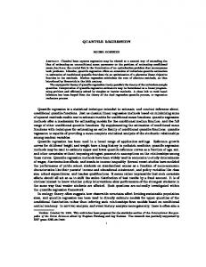
Figure 1 Illustrative Quantile Regression Example Figure 1 (Andreas Steiner, 2006) illustrates

the

quantile

regression

technique. The x and y axes represent any two variables being compared (such as age and height; or market returns and individual asset returns). The 50% quantile (middle line) is the

median, where 50% of observations fall below the line and 50% above. Similarly, the 90% quantile (top line) is where 10% of observations lie above the line, and 10% quantile (bottom line) has 90% of observations above the line. The intercept and slope are obtained by minimising the sum of the asymmetrically weighted residuals for each line. The quantile regression technique allows direct modelling of the tails of a distribution rather than ‘average’ based techniques such as ordinary least squares or credit models which focus on ‘average’ losses over a period of time. The technique has enjoyed wide application such as investigations into wage structure (Buschinsky, 1994; Machado & Mata, 2005), production efficiency (Dimelis & Lowi, 2002), and educational attainment (Eide & Showalter, 1998). Financial applications include Engle & Manganelli (2004) and Taylor (2008) to the problem of Value at Risk (VaR) and Barnes and Hughes (2002) who use quantile regression analysis to study CAPM in their work on stock market returns. In a stock market context Beta measures the systematic risk of an individual security with CAPM predicting what a particular asset or portfolio’s expected return should be relative to its risk and the market return. The lower and upper extremes of the distribution are often not well fitted by OLS. Allen, Gerrans, Singh, & Powell (2009), using quantile regression, show large and sometimes significant differences between returns and beta, both across quantiles and through time. These extremes of a distribution are especially important to credit risk measurement as it at these times when failure is most likely. We therefore expand these quantile techniques to credit risk by measuring Betas for fluctuating assets across time and across quantiles, and the corresponding impact of these quantile measurements on DD, PD and capital, as outlined further in the following methodology section.

5. Data and Methodology We use all banks listed on the Tokyo Stock Exchange for which data is available on Datastream (69 Banks in total as per Appendix 4). These banks have a market cap of USD$275 billion and assets of $8.5 trillion. Data is obtained for 10 years. We have split the data into 2 periods to compare how the banks were affected during the GFC as compared to pre-GFC. The GFC period includes the 3 years from January 2007 - December 2009. The pre-GFC period includes the 7 years from January 2000 – December 2009. 7 years aligns

with the Basel II advanced method for measuring credit risk. The early years of this period include the latter years of the Asian Financial crisis as well as the ensuing recovery period. These are the 7 years that a bank, under the advanced model, would have used to measure credit risk (and determine capital requirements) going into the GFC, usually based on the average risk over that period. By comparing this to the actual GFC data, we can determine how adequate these capital requirements would have been. In addition to the pre-GFC and GFC periods, we also measure 2008 as a single year. This year was the height of the GFC, and as it is during the most extreme period that banks are likely to fail, it is important that we isolate and measure extreme periods. We calculate DD and PD for each bank for each period using the methodology outlined in Section 3, with our “All Bank” figures being asset weighted averages. Quantiles for each period are calculated as per Section 4, with two fundamental differences. Firstly, quantile Beta analysis is normally applied to share prices, whereas we are using daily market asset values (calculated as per the methodology in Section 3). Secondly, Betas for shares are normally measured as returns of an individual share against the market. We instead are comparing risk measurements between two different periods (e.g. GFC v pre-GFC) and between different quantiles within those periods. Here we introduce the new concept of a benchmark DD (together with the associated PD and asset value standard deviation), so that we can ascertain what buffer capital is needed when asset values fall below that benchmark. To explain this concept, assume that a bank (or regulator) deems that the aggregate bank capital (leverage) ratio was adequate based on the 7 year pre-GFC asset volatility, and sets this as the benchmark capital (K). Our modelling in this study shows that the DD for this period was 3.276 (see table 2 for a year by year breakdown) which has an associated and a PD of 0.058%. At this point capital (equity ratios) of banks were approximately 5% and we will assume this is set as the benchmark. In its simplest form the Merton model is essentially a measure of capital (assets – liabilities) divided by the standard deviation of asset values. As volatility increases, DD (and hence capital) reduces proportionately. As asset value volatility is the denominator of the Merton model, a doubling of volatility ( 2/

1

= 2) means that DD

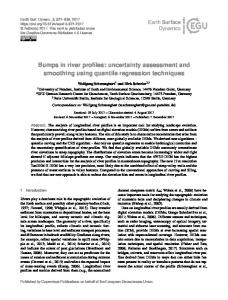
and capital (K) halve, and capital will have to be doubled (i.e. a capital buffer of 5% held) to restore the benchmark DD back to its original value. Thus any asset fluctuations and increase in DD above the benchmark value require a corresponding percentage increase in capital. We can therefore measure the extent of capital buffers required to counter extreme fluctuations as:

Required Capital Buffer = ( 2/

1 K)

-K

(4)

The capital buffer will have a minimum of zero as capital should not fall below the benchmark. The benchmark is illustrated in Figure 2, which shows a situation where the capital benchmark is 5% and actual volatility (and hence DD) has increased by 1.7x benchmark ( 2/

1=

1.7).

Figure 2 Illustration of Required Capital Buffer Using a Benchmark

!!

$ " ! # ! ' (' ) * ) +

"" !! ##

%% &

!

In this study, we measure the asset value fluctuations occurring in various quantiles of the GFC period against the pre-GFC benchmark. To allow measurement of the GFC period (or any other period within the 10 year sample period used) against the benchmark, we need a benchmark which covers the entire 10 years. We achieve this by bootstrapping the 7 year preGFC returns and extending them to 2009. We use F tests to test for volatility between the benchmark and each quantile (results for these are discussed in Section 6 and shown in Appendices tables 1b, 2b and 3b) for each selected period and bank, and between each quantile within each selected period (results discussed in Section 6 and shown in Appendices tables 1c, 2c and 3c). F is

2

2/

2

1,

whereby a value of 1 shows no difference between the two

samples measured (e.g. difference in variance between two quantiles) and a value of 3 shows variance of 3x higher for one of the two samples than the other. We use * to denote significance at the 95% level and ** at the 99% level.

In addition to using the aggregated position for all 69 banks (for which we use asset weighted averages to obtain the total DD and PD for all banks), we select one Regional and one Major bank to illustrate how quantile regression applies to individual banks. When referring to “All Japanese Banks “ in this study we are referring to the 69 banks in our study. The profile of the two example banks is given in the following two paragraphs. Sumitomo Mitsui Financial Group (SMFG) is the holding company for Sumitomo Mitsui Banking, which is one of Japan' s largest banks (along with Mitsubishi UFJ and Mizuho). The bank' s operations include retail, corporate, and investment banking; asset management; securities trading; and lending. Sumitomo Mitsui Banking has some 500 domestic branches and another 20 branches abroad. Other units of SMFG include credit card company Sumitomo Mitsui Card, brokerage SMBC Friend Securities, management consulting firm Japan Research Institute, and Sumitomo Mitsui Finance and Leasing. In the US it operates the California-based Manufacturers Bank. The bank had total assets of US 1.3 trillion at March 2010 Financial year end, a total capital ratio of 15.02% and a tier I ratio of 11.15%. Out of the three mega Japanese banks, Sumitomo Mitsui has the highest total capital adequacy ratio. Shizuoka Regional Bank is headquartered in Shizuoka, Shizuoka Prefecture. It has 187 domestic branches, primarily concentrated in the Tokai region between Tokyo and Osaka and overseas offices in Los Angeles, New York, Brussels, Hong Kong, Shanghai, and Singapore. Shizuoka Bank' s total assets stood at US$96,7 billion at March 2010 with loans and bills discounted of US $64,6 billion. The bank' s capital adequacy ratio at the same time was 15.32%, one of the highest ratios among Japanese banks, and it’s Tier I ratio was 14.06%, substantially higher than the BIS standard of 8%.

6. Results Table 2 shows how DD and PD differ from year to year of our 10 year sample period. 2001 and 2002 were periods of high volatility for Japanese banks, although as noted in the introduction section, much of the downturn in equity and asset values arising from the Asian Financial Crisis, had already occurred prior to year 2000. The mid 2000’s were a period of low volatility and default probabilities, with 2008 (the height of the GFC) showing a substantial increase in risk as indicated by these measures, reducing again in 2009.

Table 2 Annual DD and PD for All Japanese Banks from 2000 - 2009 Year 2000 2001 2002 2003 2004 2005 2006 2007 2008 2009

DD 4.20 2.07 2.21 6.99 5.71 8.36 5.85 2.78 0.99 2.77

PD