Behavior Research Methods, Instruments, & Computers 1999,3/ (4), 712-717
Using nonlinear regression to
estimate parameters ofdark adaptation GERALD McGWIN, JR., GREGORY R. JACKSON, and CYNTHIA OWSLEY
University of Alabama, Birmingham, Alabama
An objective technique jor estimating the kinetics of dark adaptation is presented, with which one can evaluate models with multiple parameters, evaluate several models oj dark adaptation simultaneously, and rapidly analyze large data sets. Another advantage is the ability to simu~ taneously estimate transition times and rates oj sensttivity recovery. Finally, this nonlinear regression te~h nique does not require that the distributional properties ofthe data be transjormed, and thus, parameter estimates are in meaningful units and rejlect the actual rate of recovery of sensitivity. In recent years, researchers have shown renewed interest in using dark adaptometry as a tool with which to investigate the mechanisms of aging (e.g., Coile ~ Bak~r, 1992; Jackson, Owsley, & McGwin, 1999), retinal disease (e.g., Brown, Adams, & Coletta, 1986; Cide~i~an, Pugh, Lamb, Huang, & Jacobson, 1997; Holopigian, SeipIe, Greenstein, Kim, & Carr, 1997; Jacobson et al., 1995), and phototransduction (e.g., Cideciyan et al., 1998; Lamb, Pugh, Cideciyan, & Jacobson, 1997; Leibrock, Reuter, & Lamb, 1998). However, as we will discuss below, there are significant challenges in estimating the critical parameters of dark adaptation from data. Dark adaptation is the recovery oflight sensitivity by the retina in the dark following exposure ofthe photopigment to intense light (Barlow, 1972; Hecht, 1937). The typical dark adaptation paradigm consists of exposing the subject to a preadapting light, followed by measuring thresholds in the dark for 30--40 min. The dark adaptation curve is produced by plotting log sensitivity as a function oftime, as is illustrated in Figure 1, and is a biphasic function. Sensitivity is expressed in terms oflog I 0 of sensitivity, since the relationship between the input to the receptor (i.e., light intensity) and the reccptor output is a logarithmic one (see Cornsweet, 1970). The first and faster phase of dark adaptation represents the cone-mediated contribution. The slower and longer second phase of the dark adaptation function is the rod-mediated contribution. The inflection point between the two phases is known as the rod-cone break, which represents the point in time during dark adap-
This research was funded by National Institutes of Health Grants ROI AG04212 and T32 EY07033, by a department grant from Research to Prevent Blindness, Inc., and by the Alabama Eye Institute. Correspondence concerning this article should be addressed to C. Owsley, Department ofOphthalmology, School ofMedicine, University of Alabama, 700 S. 18th SI., Birmingham, AL 35294-0009 (e-mail: owsley@ eyes.uab.edu).
Copyright 1999 Psychonomic Society, Inc.
tation at which the recovering rods' sensitivity surpasses the cones' sensitivity. Recent advances in our understanding of the mechanisms underlying dark adaptation have identified additional biologically relevant parameters of dark adaptation, such as the time constants of the second and third components ofrod-mediated dark adaptation (Leibrock et al., 1998). The rates of recovery of sensitivity during the second and third component of dark adaptation are largely dictated by the rate ofrhodopsin regeneration, as has been indicated by electrophysiological work on animal models (Baylor, Matthews, & Yau, 1980; Dow~in~, 19?0; Lamb, 1980, 1981) and retinal densitometry findings in humans (Rushton, Campbell, Hagins, & Brindley, 1955). On the basis ofthese findings, a biologically plausible model of dark adaptation can be constructed to describe the sensitivity recovery of the visual system during dar~ adaptation. This model consists of a single exponential representing the cone-mediated sensitivity recovery and two linear components representing the second and third components of rod-mediated sensitivity recovery. The rodcone break and the transition point in time between the second and the third components must also be estimated. Quantifying parameters of dark adaptation on the basis ofthese biologically based, multicomponent models can be difficult. This is primarily attributable to the fact that it is necessary to solve for several parameters simultaneously, each ofwhich is dependent on the other parameters to be solved. Furthermore, the statistical models used to solve for these parameters are not mathematically simple (as in a single-exponential decay; see Hahn & Geisler, 1995), because, in the present situation, we are simultaneously fitting the time constants of three components and two transition points. Furthermore, this analytic problem cannot be easily solved with popular off-the-shelf, curvefitting software. For these reasons, it is not surprising that the literature on dark adaptation is devoid of studies using sophisticated analytic techniques for identifying component parameters. We developed a non linear regression modeling technique for estimating parameters of dark adaptation that overcomes these problems and can be easily implemented. Not only does this technique minimize experimenter bias, but it facilitates the analysis of large sampie studies, such as those addressing development or aging trends or those used in c1inical trials on retinal dysfunction. Especially in the case of c1inicaltrials, one needs a standard and objective methodology that can be used with a wide range of patients with varying disease severity. Application ofNonlinear Regression to Dark Adaptation Data The goal of nonlinear regression is to fit a model to a set of data (Bard, 1974; Gallant, 1975; McCullagh & Neider, 1983). This is a more general approach than those of other types of regression models (e.g., linear regres-
712
NONUNEAR REGRESSION AND DARK ADAPTATION
o Rod-Gone Break
2 .~
..>." '00
5j3
cn
Cl
.3
\
~& ü
•
Gone-mediated
&
2nd Gomponent
•
3rd Gomponent
&
4
5
~ ~1.
.
, .•..• ,".
•
6-t--.--,.-.--,-s,.--,...-...--.--.--.,........,......,.--r--r.....-...,-...-r--r--, o 5 10 15 20 25 30 35 40 45 50 Time (Minutes)
Figure l. Typical dark adaptation curve illustrating different underlying components ofthe dark adaptation process.
sion), wherein one is applying a specific, preconceived model to a set of data. Nonlinear regression can fit data to any equation that defines Yas a function of X and one or more variables. It finds the values of those variables that generate the curve that comes closest to the data. More precisely, the goal is to minimize the sum ofthe squares of the vertical distances of the points from the curve. The application of nonlinear regression to dark adaptation data offers several features that are well suited for analyzing this type of data. Nonlinear regression allows for the use of data expressed in terms of its actual distribution. This can be done because it is possible to specify the exact form of an equation, rather than attempting to manipulate the data (e.g., changing the data's distributional properties through transformation) to fit the form of an equation. For example, it is not uncommon for researchers to mathematically transform data to make it fit a Gaussian distribution, so that linear models can be applied to it. A more appropriate approach would be to use the actual, untransformed data and develop a regression model that reflects the true structure of the data. Therefore, parameter estimates are in meaningful units and do not require back transformations for interpretation purposes. Another feature of nonlinear regression is the ability to simultaneously estimate transition times and rates of recovery free of experimenter bias. It can accomplish this by treating such parameters as variables in the model and iteratively solving for them until a specified stopping point (usually, until adjustments make virtually no difference in the sum of squares). Finally, any model of dark adaptation based on a theoretical or a biological construct
713
that can be expressed mathematically can be estimated with this technique. To implement this nonlinear regression technique, we used SAS (SAS Institute, Cary, NC). Although a number of other software packages (e.g., Matlab [The Mathworks, Inc., Natick, MA], S-Plus [MathSoft, Inc., Cambridge, MA]) could have been used, SAS was chosen for the following reasons. First, SAS is a popular and widely used software package in the behavioral sciences. Second, using built-in statistical procedures, we were able to easily implement the nonlinear regression portion of the program. Third, SAS is a cross-platform software package (e.g., PC, Macintosh, Unix), making this program easily implemented in numerous computing environments without modification. Fourth, SAS offers a flexible framework that allows the evaluation of multiple models without extensive modification to the analysis program. Description of the Program The data input (see the program listing in the Appendix) portion of the program reads a tab-delimited text file specified by the infile command. The order of the variables in the file is subject identification number (ID), time (MIN), and log threshold (THRESH). The program initialization portion of the program creates temporary variables and conducts preliminary calculations to be used later in the program. The model initialization portion of the program conducts a preliminary linear regression analysis. In SAS, the non linear regression procedure requires that the user supply the initial values for parameter estimates. This is accomplished by using the results of a preliminary linear regression. The preliminary linear regression models the dark adaptation data, using four linear components. The user chooses the four linear components as delimited by the inputted transition points. These points are fixed and are not explicitly solved as part ofthe analysis. An alternative approach would have been to exclude the preliminary linear regression modeling and fix the initial values for the nonlinear regression procedure. However, the drawback ofthis alternative is apparent when there is large individual variability in the data (e.g., normal vs. those with retinal disease). By running the linear regressions individually for each subject, the resulting nonlinear regressions are provided initial values that are specific to that subject, thereby reducing computing time by decreasing the number of computational iterations necessary to solve for the final nonlinear model parameters. The nonlinear regression portion ofthe program contains four statements for each model evaluated. The resulting values from the linear regression model are used to initialize the parameter estimates in the PARMS statement of the PROC NUN procedure. The preliminary transition times (KNOTS) are specified by the user. It should be noted that these KNOT values are solved as part ofthe model estimation procedure and are not treated as fixed values. For estimation ofthe model parameters, the
714
McGWIN, JACKSON, AND OWSLEY
o
- - Two Exponential Component Model - - - Single Exponential, Two Linear Component Model
2 .~ > EI/)
153
cn
Cl
.3
4
5
6-t-.,--r-r"""","""",......,.......,r-r"""","""",......,.......,r--r-,--.-.,...-......-,
o
5
10
15
20
25 30 Minutes
35
40
45
50
Figure 2. Dark adaptation curve from a 25-year-oldperson in good ocular health. Solid line represents the nonlinear regression fits for the two-exponential model, and dashed line represents the oneexponential, two-Iinear model.
NUN procedure uses the method of false position (also known as the doesn 't use derivatives [DUD] or secant method; Ralston & Jennrich, 1978). One could also use a number of other estimation procedures, inciuding GaussNewton, Marquardt, steepest descent (gradient), and Newton (Bard, 1974; Hartley, 1961; Marquardt, 1963). To use the Gauss-Newton method, delete the METHOD= DUD option in the PROC NUN statement. Our evaluation ofthese methods indicated that they produced equivalent results, with the method offalse position requiring slightly fewer iterations. The MODEL statement is the mathematical expression of the dark adaptation model. The NUN procedure iterates a maximum of 200 times. Estimation of model parameters will cease when the change in the sum of squared errors from iteration/ - 1 to iteration/ is 10- 8 or less. The r 2 value is also calculated for each model. Finally, the subject number, solved parameters, and r 2 value are output to the screen. In the case of multiple subjects, the program then processes the next subject's data. Examples We demonstrate the application of non linear regression on data from two observers, a 25-year-old and a 75year-old, both in good ocular health. Two models of dark adaptation are applied to each subject's data: a ciassic two-exponential-component model [y = (a + b * exp(-c * x)) + (d * exp(-e * ([max(x - knotl,O)]))); Barlow, 1972; Hecht, 1937] and a single-exponential, two-linearcomponent model of dark adaptation [y = +b* exp (-c * x)) + (d * ([max(x - knotl,O)]))) + (e *
«a
([max(x - knot2,0)])); based on Lamb, Cideciyan, Jacobson, & Pugh, 1998, and Leibrock et al., 1998]. Figure 2 presents log sensitivity as a function oftime after the bleach for the 25-year-old adult. This data is representative of adults in their 20s (Jackson et al., 1999). The nonlinear regression program was applied to the data; the solved non linear regression equations for both the two-exponential-component model (solid line) and the one-exponential, two-linear-component model (dashed line) are plotted. The equation for the former model isy = 51.71 + (-19.78 * exp(-0.85 * x)) + (-30.94 * exp(-0.12 * (MAX(x - 13.32,0)))), with an r 2 value of .99. For the latter model, the equation is y = 20.49 + (-19.86 * exp( -0.91 * x)) + (2.17 * (MAX(x 12.23,0))) + (-1.81 * (MAX(x - 23.06,0))). This model had an r 2 value of .99. Both models fit the data weil, as is evidenced by the high r 2 values. A z test can be used to determine whether one model provides a significantly better fit to the data. There was no evidence that either model fit the data better (z = 0.06, P > .05). Dark adaptation data and solved nonlinear regression equations for the 75-year-old subject are presented in Figure 3. Respectively, the equations for the two-exponentialcomponent model and the one-exponential, two-linearcomponent model are y = 47.87 + (-15.68 * exp( -0.2 * x)) + (-29.78 * exp(-0.09 * (MAX(x - 18.32,0)))) and y= 14.65 + (- 398.54 * exp( -1.77 * x)) + (1.54 * (MAX(x - 14.21,0)))+ (- 1.28 * (MAX(x - 31.4,0))). As is evident from Figure 2, the two-exponential-component model does not appear to fit the data as weil as the one-exponential, twolinear-component model. This is supported by the higher r 2
o
- - Two Exponential Component Model - - - Single Exponent/al, Two Linear Component Model
. ....... ........,;;: ... •
5
•
0,""""
6 -t-,.....,...,.....,,.,...,...,-,-...........,...,........,-r--r-...,..,--.-,...,..,....,.......,....,....,
o
5
10 15 20 25 30 35 40 45 50 55 60 65 Minutes
Figure 3. Dark adaptation curve from a 75-year-old person in good ocular health. Solid line represents the nonlinear regression fits for the two-exponential model, and dashed line represents the oneexponential, two-Iinear model.
NON LINEAR REGRESSION AND DARK ADAPTATION value forthe one-exponential, two-linear-component model (.99), as compared with that ofthe two-exponential-component model (.92). The one-exponential, two-linear-component model fits the data better than does the two-exponential-component model (z = 5.77, p < .001). The values for the transition times are available directly from the program output. For example, for the twoexponential-component model for the 75-year-old subject, the transition time was 18.32 min. To obtain rates of sensitivity recovery, simple mathematical calculations are performed on the parameter estimates. The nature of these calculations are dependent on the form ofthe dark adaptation model chosen.
Availability Interested users who prefer not to type in the programs can request an ASCII file ofthe program by e-mailing the first author (
[email protected]). REFERENCES BARD. J. (1974). Nonlinear parameter estimation. New York: Academic Press. BARLOW. H. B. (1972). Dark and light adaptation: Psychophysics. In D. Jameson & L. M. Hurvich (Eds.), Handhook ofsensory physiology (Vol. VII, pp. 1-28). New York: Springer-Verlag. BAYLOR. D. A.. MATTHEWS. G.. & YAU. K. W. (1980). Two components of electrical dark noise in toad retinal rod outer segments. Journal of Phvsioiogy, 309. 591-621. BROWN. B.. ADAMS. A. J.. & COLETTA. N. J. (1986). Dark adaptation in age-related maculopathy. Ophthalmologie & Physiologie Optics, 6, 81-84. CIDEClYAN, A. v.. PUGH. E. N.. LAMB. T. D.. HUANG. Y.. & JACOBSON. S. G. (1997). Rod plateau during dark adaptation in Sorsbys fundus dystrophy and vitamin A deficiency. Investigative Ophthalmology & Visual Science, 38, 1786-1794. CIDEClYAN. A. v.. ZHAO, X. Y.. NIELSEN. L., KHANI. S. C. JACOBSON, S. G.. & PALCZEWSKI. K. (1998). Null mutation in the rhodopsin kinase gene slows recovery kinetics of rod and cone phototransduction in man. Proceedings ofthe National Academv ofSciences, 95, 328-333. COILE. CD., & BAKER, H. D. (1992). Foveal dark adaptation, photopigment regeneration, and aging. Visual Neuroscience, 8, 27-29.
715
CORNSWEET, T. N. (1970). Visual perception, New York: Acadcmic Press. DOWLlNG,1. E. (1960). The chemistry of visual adaptation in the rat. Nature, 188, 114-118. GALLANT. A. R. (1975). Nonlinear regrcssion. American Statistician, 29, 73-81. HAHN. L. W, & GEISLER. W S. (1995). Adaptation mechanisms in spatial vision: 1. Bleaches and backgrounds. Vision Research. 35, 15851594. HARTLEY. H. Ü. (1961). The modified Gauss-Newton method for the fitting of nonlinear regression functions by least squares. Technometrics, 3, 269-280. HECHT. S. (1937). Rods, cones, and the chemica1 basis ofvision. Physiological Review, 17,239-290. HOLOPIGIAN, K., SEIPLE. W, GREENSTEIN, v.. KIM, D., & CARR. R. E. (1997). Relative effects of aging and age-related macular degeneration on peripheral visua1 function. Optometry & Vision Science, 74. 152-159. JACKSON. G. R., ÜWSLEY, C. & MCGWIN. G. (1999). Aging and dark adaptation. Vision Research, 39, 3975-3982. JACOBSON, S. G., CIDECIYAN, A. v.. REGUNATH. G., RODRIGUEZ, F. J.• VANDENBURGH, K.. SHEFFlELD. V. C. & STONE, E. M. (1995). Night blindness in Sorsbys fundus dystrophy reversed by vitamin A. Nature Genetics, 11.27-32. LAMB, T. D. (1980). Spontaneous quantal events induced in toad rods by pigment bleaching. Nature, 287, 349-351. LAMB. T. D. (1981). The invo1vement of rod photoreceptors in dark adaptation. Vision Research. 21. 1773-1782. LAMB, T. D., CIDEClYAN, A. v.. JACOBSON, S. G., & PUGH, E. N. (1998). Towards a molecular dcscription ofhuman dark adaptation. Journal o{ Physiology, 506, 88P. LAMB, T. D., PUGH, E. N.• CIDECIYAN. A. v.. & JACOBSON, S. G. (1997). A conceptual framework for analysis of dark adaptation kinetics in normal subjects and in patients with retinal disease. Investigative Ophthalmology & Vision Science, 38(Suppl.), S 1121. LEIBROCK, C S.• REUTER, T., & LAMB. T. D. (1998). Molecular basis of dark adaptation in rod photoreceptors. Eye, 12,511-520. MARQUARDT, D. W. (1963). An algorithm for least squares estimation ofnonlinear parameters. Journalfor the Society ofIndustrial & Applied Mathematics, 11, 431-441. MCCULLAGH. P.• & NELDER. J. A. (1983). Generalized linear models. London: Chapman Hall. RALSTON, M. L., & JENNRICH, R. I. (1978). DUD. a derivative-free algorithm for nonlinear least squares. Technometries. 20, 70-74. RUSHTON. W. A. H.• CAMPBELL, F. W.• HAGINS, W. A.. & BRINDLEY, G. S. (1955). The bleaching and regeneration of rhodopsin in the living eye ofthe albino rabbit and ofman. Optical Acta, 1. 183-190.
(Continued on next page)
716
McGWIN, JACKSON, AND OWSLEY APPENDIX Program Listing **************************************************************************************., *., * THIS PROGRAM FITS 3 SEPARATE MODELS TO DARK ADAPTATION DATA. *., * INPUT DATASETS MUST INCLUDE VARIABLES NAMED "X" AND "Y". *. STARTING ESTIMATES FOR MODEL I ARE CALCULATED FROM PIECEWISE LINEAR , * *., * MODEL AND DO NOT NEED TO BE MODIFIED. KNOT MODIFICATIONS MAY BE * NECESSARY. STARTING ESTIMATES FOR MODELS 2 AND 3 MAY REQUIRE * MODIFICATION DEPENDING ON AMOUNT OF DATA AVAILABLE AND FIT OF ASSUMED *; *., * MODELS. LOG FILE SHOULD BE MONITORED FOR CONVERGENCE PROBLEMS, *., * DEFAULT IS (MAXITER=300) *., * *., * MODEL I: I EXPONENTIAL COMPONENT & 2 LINEAR COMPONENTS *. y=«a+b*exp(-c*x))+(d*([max(x-knot 1,0)))))+(e*([max(x-knot2,0))) , * *., * *., * MODEL 2: 2 EXPONENTIAL COMPONENTS *., * y=(a+b*exp(-c*x))+(d*exp( -e*([max(x-knot 1,0)]))) *. , * *., * EACH MODEL USES PROC NLIN TO SOLVE THE PARAMETER ESTIMATES AND *., * KNOTS. OUTPUT CAN BE USED TO SOLVE EACH OF THE ABOVE EQUATIONS. *., * *., * * WRITTEN BY: GERALD MCGWIN, JR. OCTOBER 1998 *; **************************************************************************************., /***************~**********************************
DATA INPUT PORTION OF PROGRAM **************************************************/ data one; infile "c:\ testdata.txt" expandtabs missover; input ID MIN THRESH; /************************************************** PROGRAM INITIALIZATION PORTION OF PROGRAM **************************************************/ xx_I = max(x - 1.0, xx_2 = max(x - 10.0, xx_3 = max(x - 20.0,
0); 0); 0);
%macro passest; proc univariate noprint; var y; output out=tss_temp mean=ave; data _null_; set tss_temp; call symput('ave',put(ave,12.6)); data aa; set one; temp = (y - &ave)**2; proc univariate noprint; var temp; output out=tss sum=tss; data _null_; set tss; call symput('tss',put(tss,8.6)); proc reg noprint data=one outest=reg_est; model y = x xx_1 xx_2 xx_3; data _null_; set reg_est; call call call call call
symput('bO',put(intercep,5.2)) ; symput('b I ',put(x,5.2)) ; symput('b2',put(xx_I,5.2)) ; symput('b3',put(xx_2,5.2)) ; symput('b4',put(xx_3,5.2)) ;
/************************************************** NONLINEAR REGRESSION PORTION OF PROGRAM **************************************************/
NON LINEAR REGRESSION AND DARK ADAPTATION APPENDIX (Continued)
**********., proc nlin noprint maxiter = 300 method = dud data=one outest=nlin_est ; parms a=20 b=-20 c=0.90 d=2.1 0 e=0.40 knot I= I0 knot2= 23 ; xxi = max(x-knotl,O); xx2 = max(x-knot2,0); model y = (( a + b*exp(-c*x» + (d*(xxl») + (e*(xx2»; data nlin_est; set nlin_est; if _type_ = "FINAL"; drop _name__iter_; model = "I EXP&2LINE";r2=I-Lsse_/&tss); proc print data-nlin cst ; **********., proc nlin noprint maxiter = 300 method = dud data=one outest=nlin_est; parms a=50 b=-20 c=0.8 d=IO e=0.2 knotl=I5; xx = max(x-knot I, 0); model y = (a + b*exp(-c*x» + (d*exp(-e*(xx))); data nlin_est; set nlin_est; if _type_ = "FINAL"; drop _name__iter_; model = "2 EXPONENTIALS"; r2=I-Csse_/&tss); proc print data=nlin_est;
**********., %mend passest; %passest run;
(Manuscript received November 3, 1998; revision accepted for publication March 26, 1999.)
717