radio-modes are assigned to at least th nodes in the map. Assume that the advertised radio-modes are. {rmi1, rmi2, ..., rmij}. Node v computes the probabil-.
Using Reconfigurable Radios to Increase Throughput in Wireless Sensor Networks Mihaela Cardei and Yueshi Wu Department of Computer and Electrical Engineering and Computer Science Florida Atlantic University Boca Raton, FL 33431, USA E-mail: {mcardei, wuy2013}@fau.edu Abstract—In traditional wireless sensor networks communicating on a single channel the data throughput measured at the sink is constrained by the radio capability, contentions, and collisions, which increase in the region closer to the sink. Using SDR technology, different levels of configuration within a transceiver are allowed. In this paper we assume that the sink and sensor nodes are equipped with reconfigurable radios. We design a distributed algorithm used by sensor nodes to reconfigure their radio according to some predefined radio-modes, such that the resulting topology is connected to the sink. Collecting sensor data using this topology reduces the interference and increases the network throughput and the data delivery rate. We analyze the performance of our algorithm using ns-3 simulations. Keywords: wireless sensor network, radio-mode assignment, multi-radio sink, distributed algorithm.
I. I NTRODUCTION AND R ELATED W ORKS A wireless sensor network (WSN) consists of sensor nodes that are densely deployed either inside the phenomenon or very close to it. Sensor nodes measure various parameters of the environment and transmit collected data to the sink. Once a sink received sensed data, it processes and forwards them to the users. The nodes closer to the sink are involved in more data transmissions and they consume more energy than sensors deployed farther away from the sink. This is because, besides their own packets, they forward packets on behalf of other sensors. When the whole WSN communicates on only one channel, the data throughput measured at the sink is constrained by the radio capability, contentions, and collisions which increase in the region closer to the sink. These lead to retransmissions and packets being dropped. With the development of Software Defined Radio (SDR) technology, different levels of reconfiguration within a transceiver are allowed. Multi-band, multichannel, multi-standard, multi-service systems can be achieved with SDR. Cognitive radios enable WSNs to use vacant licensed channels. The advanced technology makes multi-channel communication realistic.
A cognitive radio can be programmed to transmit and receive on a variety of frequencies and to use different transmission technologies supported by its hardware design. A radio is reconfigurable if it has the capability to adjust its transmission parameters on the fly, without any modifications to the hardware. These parameters include spectrum band, transceiver parameters, and modulation scheme. Cognitive radio networks can operate in both licensed and unlicensed bands [1]. When operating on licensed bands, the objective is to exploit spectrum holes through cognitive communication, giving priority to the primary users. In unlicensed bands, all users have the same priority. ISM bands are used nowadays by many radio technologies and has started to decrease in efficiency with an increase in interference. Cognitive radio networks can be used to increase efficiency and QoS through intelligent spectrum sharing. Our work fits in this category. We propose a distributed algorithm that improves network performance through spectrum sharing. Many approaches proposed for traditional multichannel WSNs mainly focus on reducing the interference caused by simultaneous transmissions. Most of the works are exploiting the 802.15 channels. A treebased multichannel scheme is proposed in [3]. This approach partitions the network into different subtrees communicating on different channels thus eliminating the inter-tree interference. First, a fat tree routed at the base station is computed based on the breadth first search algorithm. Then channels are allocated from top to bottom, partitioning the network into different subtrees communicating on different channels. In our work we assume that sensor nodes can reconfigure their radios to some predefined radio-modes selected by the sink. A radio-mode is characterized by spectrum band, communication parameters, and modulation scheme. Thus different modes may have different communication ranges and different transmission data rates. This aspect was not accounted for in [3]. In addition, in our algorithm data collection is not performed at the same time as the radio-mode selection.
k.
Another tree-based joint channel selection and routing scheme is proposed in [4], which aims to improve the network lifetime by reducing the energy consumed on overhearing. Beacon messages containing the receiver channel are sent on different channels in rotation. The receiver channel is chosen to be the least used channel between neighbors after a random backoff though a common default channel. The transmit channel is chosen dynamically based on the battery health among all upstream nodes. All nodes listen on the receiver channel and switch to the transmit channel for data transmission. Data may be transmitted on different channels at each hop thus the overhearing is minimized. This approach leads to a frequent channel switching and to a restricted broadcast. An application based clustering mechanism is proposed in [5]. Nodes with similar sensed data (e.g. temperature) are assigned to the same channel, forming a data plane. It is assumed that geographical proximity implies high data correlation. Cluster heads (CHs) in each data plane and the sink communicate though a common control channel while sensor nodes send data to their CH though the assigned intra-cluster channel. The application dependent assumption makes this approach hard to extend for different sensing mechanisms. The remainder of the paper is organized as follows. Section II presents motivation and we formally define the radio-mode assignment for increased throughput in WSNs problem. In Section III we propose a distributed algorithm whose performance is simulated in Section IV. Section V concludes the paper. II. M OTIVATION
AND
The objective is that sensor nodes assign radio-modes to their radios such that the resulting topology is connected and data throughput is increased. Radio-Mode Assignment for Increased Throughput in WSNs (RMA) Problem: Given a WSN with n sensors and a sink S, where each sensor has 1 reconfigurable radio and the sink has k reconfigurable radios, assign to each radio a radio-mode from the set C = {rm0 , rm1 , ..., rmm−1 }, m ≥ k, such that the resulting topology is connected and the throughput is increased assuming a high data traffic application. III. D ISTRIBUTED A LGORITHM P ROBLEM
FOR THE
RMA
In this section we present our solution for the RMA problem. Different radio-modes are illustrated in section III-A. The objective is that each sensor node assigns its radio to a radio-mode such that the overall topology is connected.
Fig. 1.
P ROBLEM D EFINITION
Network Organization
We propose the network organization from Figure 1. The sink S is equipped with k radios and chooses k radio-modes from the set C. Let us denote the set of radio-modes selected by the sink with Csink , where Csink ⊆ C. The sink assigns each radio a radio-mode from Csink . All the sensor nodes in the network assign their radios to rm0 during phases 1 and 2. rm0 ∈ Csink is the radio-mode with the smallest transmission range (and the highest frequency). In the phase 1, the sink broadcasts a message containing Csink by flooding. In the phase 2, the nodes are involved in a distributed algorithm during which each sensor node selects a radio-mode from Csink such that the overall topology remains connected. Each sensor assign its radio to the selected radio-mode at the end of phase 2. Phase 3 is the data gathering phase. Data is generate by sensor nodes and collected by the sink. The overall topology contains t connected topologies using different radio-modes. Any data collection mechanism can be used in this phase. One such example is data collection using shortest-path trees.
The objective of this paper is to provide a mechanism that improves network capacity and data throughput. In WSNs data is collected using convergecast. The bottleneck is at the sink which receives data from a large number of sensors and in the region closer to the sink where the traffic is higher. To deal with this issue, we propose to use a sink with multiple radios. We consider a WSN consisting of n homogeneous sensor nodes s1 , s2 , ..., sn and a sink node S. We assume that sensor nodes are densely deployed and the WSN is connected. The sink node S is used to collect data and is connected to the network of sensors. Data collection follows a convergecast communication model, where data flow from many nodes (e.g. the sensors) to one (the sink). Sensor nodes are resource constrained devices, while the sink is a more resource-powerful device. Each sensor node is equipped with one reconfigurable radio and the sink is equipped with k reconfigurable radios. We assume that both the sensors and the sink can adjust the transmission parameters of their radios to radiomodes from the set {rm0 , rm1 , ..., rmm−1 }, where m ≥ 2
TABLE I C OMPARISON OF VARIOUS W IRELESS S ENSOR R ADIO -M ODES SensorMotes
TX Range
Frequency Band
Data Rate(max)
Radio Module
Mica2 [6] 868/916MHz Mica2 [6] 433MHz Mica2Dot [7] 868/916MHz MicaZ [8]
152m,outdoor
868/916MHz
38.4Kbps
CC1000
304m,outdoor
433MHz
38.4Kbps
CC1000
152m,outdoor
868/916MHz
38.4Kbps
CC1000
75-100m,outdoor
2.4GHz
250Kbps
CC2420
Waspmote [9][10] 2.4GHz Waspmote [9][11] 900MHz Waspmote [9][12] 868MHz
7000m,outdoor
2.4GHz
250Kbps
XBee-PRO-ZB
10km
900MHz
156Kbps
XBee-900
12km
868MHz
24Kbps
XBee-868
radio-mode rmi . In both steps 1 and 2 sensor nodes configure their radio to rm0 . In step 2, each sensor node selects a radio-mode from Csink , and at the end of the step 2 sensors reconfigure their radio to the selected radio-mode. The objective is that each sensor node selects a radio-mode from Csink , such that the resulting topology remains connected to the sink after sensors reassign their radios at the end of step 2. 1) Step 1- Neighbor Discovery and Setting up the Distance to the Sink: Let us denote by Nk (u) the k’th neighborhood of a node u, where Nk (u) = {v|dist(u, v) ≤ k hops}. The sink S constructs N1 (S) and N2 (S), while each other sensor node v constructs N1 (v). All the nodes including the sink S broadcast a Hello message containing the node ID. The message is sent with a small random delay to avoid collisions. After a short time interval, each node u which is 1-hop away from the sink sends a second Hello message, containing the node ID and N1 (u). Based on this information, S computes N2 (S). Each other sensor node v knows N1 (v). In the second part of this step, the sink broadcasts a message Hops which contains a parameter hops - the number of hops to the sink. A sensor node receiving a Hops message retransmits the message in two cases: (i) if this is the first Hops message received, or (ii) if this message contains a shorter distance to the sink. In both cases the node updates its shortest distance to the sink, increments the hops counter, and then retransmits the Hops message. At the end of this step, each sensor node knows its smallest number of hops to the sink using rm0 . 2) Step 2 - Radio-Mode Selection by Sensor Nodes: The number t of topologies connected to the sink S is upper-bounded by k = |Csink | and by the number of nodes in N1 (S), that is t =min{ k, |N1 (S)| }. First, the sink S assigns radio-modes to the
A. Characteristics of Radio Module of Various Sensor Platforms Wireless sensor motes are mostly equipped with dipole antennas. Compared to channels at higher frequency, those at lower frequency have better propagation characteristics and achieve larger transmission range when they use the same transmitting power. Existing commercial sensor motes operating on different channel frequencies achieve different transmission ranges and different data rates. For example, sensor motes using lower frequency bands such as 868/900 MHz achieve lower data rate than those at 2.4 GHz band and they have a larger transmission range. In Table I we examine different wireless sensor radios and compare RF modules operating at different frequencies. We can observe that sensor motes transmitting on lower frequency bands are characterized by a larger transmission range and have a smaller data rate. With the development of the SDR technology, different levels of reconfiguration within a transceiver are possible. Multi-band, multi-channel, multi-standard, multiservice systems can be achieved. Using SDR, radios can be configured to different schemes as used in the existing RF modes, according to different needs. Our construction of the t-overlapping topologies accounts for the fact that different radio-modes may be characterized by different transmission ranges. B. A Distributed Algorithm for Radio-Mode Assignment This algorithm is executed in phase 2 and has two steps: • Step 1 - neighbor discovery and setting up the distance (hop count) to the sink • Step 2 - radio-mode selection by the sensor nodes. Let us assume without loss of generality that the k radio-modes selected by the sink are Csink = {rm0 , rm1 , ..., rmk−1 }, ordered such that tx0 ≤ tx1 ≤ ... ≤ txk−1 , where txi is the transmission range of the 3
Algorithm 1 SinkAssignRadioModesN1(S)
Algorithm 3 AssignRadioMode(v) 1: if v receives a radio-mode assignment rmi in the message
1: ComputeRadioModesN1 (S) 2: broadcast SinkRMSetN1 (S, N1 (S), radio-modes assigned
2:
to the sensors in N1 (S), TTL = 1)
3:
Algorithm 2 ComputeRadioModesN1(S) 1: 2: 3: 4: 5: 6: 7:
8: 9: 10: 11: 12: 13: 14: 15: 16: 17: 18: 19: 20: 21: 22:
4: 5: 6: 7:
t = min{ k, |N1 (S)| } let Ct = {rm0 , rm1 , ..., rmt−1 } if t == |N1 (S)| then assign nodes in N1 radio-modes rm0 , rm1 , ..., rmt−1 return end if for each rmi ∈ Ct compute N rmi - number of sensors in N1 (S) with primary radio-mode rmi , such that |N rmi − N rmj | ≤ 1 for any rmi , rmj ∈ Ct U = N1 (S) for each radio-mode rmi , i = 0 to k-1 do /* assign the radio-mode rmi to N rmi nodes */ for each node x in U do x.conf l = 0 end for for i = 1 to N rmi do pick up a node x in U with the smallest x.conf l value assign x the radio-mode rmi U = U − {x} for each node y in U which is neighbor of x do y.conf l = y.conf l + 1 end for end for end for
8:
9: 10: 11:
SinkRMSetN1 then wait a random time and broadcasts RMSet(v, rmi , TTL = 1) assign the radio-mode rmi to its radio after sending RMSet return else set a waiting time twait = T ime(vhops ) record radio-modes assigned by neighbor nodes based on RMSet messages received when twait expires, v examines the recorded neighbor radio-modes and select a radio-mode, let us say rmi (see explanation in the text) wait a random time and broadcasts RMSet(v, rmi , TTL = 1) assign the radio-mode rmi to its radio after sending RMSet end if
radio-modes assigned to N1 (S), TTL = 1). Each sensor node v assigns a radio-mode using the procedure AssignRadioMode(v). If the node v ∈ N1 (S), then it receives the SinkRMSetN1 message from the sink, which contains the radio-mode selected by S for v. All other nodes assign their radio-modes in increasing order of their distance (number of hops) to the sink. Once a sensor selects its radio-mode, it broadcasts a RMSet message, informing its neighbors of its radiomode decision. After broadcasting the RMSet message, the node configures its radio to the new radio-mode selected. A node v sets up a waiting time twait during which it waits to receive messages from neighbors. twait is proportional with the distance to the sink vhops - the number of hops to the sink. The waiting time is computed as T ime(vhops ) = vhops × hopDelay, where hopDelay is the delay per hop and it must account for the propagation delay, algorithm execution time, and the maximum waiting time of a node before sending the RMSet message. In this way the nodes at distance 1 will set up their radio-mode first, followed by the nodes at distance 2, then 3, and so on. When the timer expires, the node takes a decision on selecting a radio-mode among those already advertised by the neighbors. Node v maintains a map with pairs containing node ID and radio-mode selected. The mechanism for selecting a radio-mode works as follows. First, the objective is to distribute nodes on all topologies, so that messages are transmitted simultaneously on various radio-modes. We define a threshold value th, which is a small number, for example th = 3. If the map contains radio-modes assigned to less than th nodes, then the selected radio-mode is the one assigned to the smallest number of nodes. In case of a tie, a radio-mode
sensor nodes in N1 (S) using the algorithm SinkAssignRadioModesN1(S) which is explained next. The sink computes radio-modes for the nodes in N1 (S) using the function ComputeRadioModesN1(S). If t == |N1 (S)|, then each node in N1 (S) receives a different radio-mode rm0 , rm1 , ..., rmt−1 . If |N1 (S)| > k, then t = k. There will be multiple nodes in N1 (S) with the same radio-mode assigned. Line 7 computes N rmi - the number of sensor nodes in N1 (S) to be assigned the radio-mode rmi , for i = 1 to k. The objective is to balance the number of sensors that use each radio-mode, thus |N rmi − N rmj | ≤ 1 for any rmi , rmj ∈ Ct . For example if |N1 (S)| = 10 and k = 3, then N rm0 = 4, N rm1 = 3, and N rm2 = 3. The radio-modes rm0 , rm1 , ..., rmk−1 are assigned in order. We denote by U the nodes in N1 (S) which have not been assigned a radio-mode yet. Nodes are selected from U in a greedy manner, choosing the one with the smallest conflict in each iteration. In order to update the conflict values, the information in N1 (S) and N2 (S) is needed by S. After all the nodes in N1 (S) have been assigned radiomodes, S broadcasts a message SinkRMSetN1(S, N1 (S), 4
(a) Radio-mode assignment by the sensor nodes Fig. 2.
(b) Multiple tree construction
Example of radio-mode assignment by the sensors and trees construction.
radio to rmi . The proof is by mathematical induction. Sensor nodes in N1 (S) have the radio-mode assigned by the sink, thus they are connected to the sink after switching their radio-mode. Let us consider a sensor node v. It builds a map containing pairs with neighbors and the radio-mode selected. In the inductive step, we assume those neighbors are connected to the sink using the corresponding modes. When v selects one of the radio-modes in the map, let us say rmi , it automatically becomes connected to at least one node in the map, let us call it u, which is connected to the sink on the radio-mode rmi . It should be noted that since v and u are neighbors using rm0 , they remain connected when both u and v switch to rmi since the transmission range txi ≥ tx0 . It follows that v is connected to the sink after switching to the radio-mode rmi .
is selected arbitrarily. For example, if node v has the map {(a, rm0 ), (b, rm1 ), (c, rm0 ), (d, rm2 ), (e, rm0 ), (f, rm1 )} then v selects the radio-mode rm2 . Let us consider the case when all the advertised radio-modes are assigned to at least th nodes in the map. Assume that the advertised radio-modes are {rmi1 , rmi2 , ..., rmij }. Node v computes the probability of selecting the radio-mode rmir as pir = Pj dir d , x=1 ix where r = 1, 2, .., j and dir is the data rate of the radiomode rmir . Once a radio-mode rmi is selected, node v waits a random time to avoid collisions and transmits a RMSet message to inform neighbors of its selection. At the end of this step, each sensor node v switches its radio to the selected radio-mode. Such an example is illustrated in Figure 2a, where k = 3. Each sensor node has selected one of the three radio-modes rm0 , rm1 , or rm2 . Theorem Assuming that the initial topology is connected on rm0 , at the end of phase 2, when sensor nodes configure their radios to the newly selected radio-modes, the resultant overall topology is connected. Proof: Take Figure 2a as an example first. The sink has 3 radios, each with radio-modes rm0 , rm1 , and rm2 . All sensors have assigned one of the radio-modes rm0 , rm1 , or rm2 . Sensors with rm0 form a connected topology, which is connected to the sink. The same applies to radio-modes rm1 and rm2 . We claim that sensor nodes on a certain radio-mode rmi form a connected topology, connected to the sink. First, all sensors use radio-modes among those used by the sink, so rmi must be used by the sink for one of its radios. We prove that each sensor v selecting a radio-mode rmi is connected to the sink at the time it switches its
C. Data Gathering The data gathering protocol explained in this section the uses shortest-path routing. This protocol can be replaced accordingly by a more sophisticated protocol, as required by the WSN application. As discussed in the previous sections, each sensor node has assigned one of the radio-modes rm0 , rm1 , ..., rmt−1 and the sink has k radios, where t ≤ k. The sink sends messages SetParent(S, rmi , hops = 0) on each of the t radio-modes using the transmission range corresponding to each radio-mode. The transmission range varies with the frequency: for higher frequencies the transmission range is smaller. Each sensor-node receiving the SetParent message for the first time (or with a shorter distance) sets-up its parent node (on the same radio-mode) and the number 5
of hops to the sink. Then it increments the variable hops and retransnmits the SetParent message. Figure 2b shows three resulting data collection trees, each on a different radio-mode, after each node sets up its parent. Data generated by sensor nodes flow to the sink along the t trees, using the parent node as next hop.
2000 bytes. We run each simulation scenario 5 times using different seed values and report the average values in the graphs. Each simulation scenario is run for 20 seconds. Beside the RMA algorithm, we test the case when the whole network uses the same radio-mode. For example, in the “radio-mode 0” case all the nodes assign their radio to the radio-mode 0. Data collection is performed along the shortest-paths as well. B. Simulation Results
Fig. 3.
In the first experiment we compare traditional WSNs operating on a single radio-mode. In Figure 4 we compare radio-mode 0, radio-mode 1, and radio-mode 2 when message size is 500 bytes. Figure 4a shows the data throughput or received data rate at the sink. The highest throughput is received by the radio-mode 0, followed by radio-mode 1 and radio-mode 2. These are in the decreasing order of the data-rate of the corresponding modes. As the network becomes overloaded, queuing delays increase, triggering packets to be dropped. Figure 4b shows the end-to-end delay which is computed as the average of the end-to-end delay of the messages received by the sink. Radio-mode 2 has the highest delay, followed by radio-mode 0 and radiomode 1. The delays for the radio-modes 0 and 1 are comparable, and they are much smaller than the delay of radio-mode 2. The higher delay of radio-mode 2 with the data rate of 1 Mbps is due to the high queuing delays. The delivery ratio measurements in Figure 4c is consistent with the throughput results, showing a higher delivery ratio for radio-mode 0, followed by radio-modes 1 and 2. For each mode, p = 100 has a higher throughput initially, but as the network becomes overloaded, p = 30% produces a higher throughput. The end-to-end delays are higher for p = 100% since the queuing delays are higher. The delivery ratio is higher for p = 30% since fewer packets are being dropped. In the second experiment in Figure 5 we compare the four algorithms when we vary the message size M sgSize = 100, 250, 500, 750, 1000, 1250, 1500, 1750, 2000 bytes. The number of sensors is n = 1323, p = 100%, and the data generation interval is 1 sec. The aggregate network load on the x-axis is computed as M sgSize ∗ 8 ∗ n/(interval ∗ 106 ) Mbps. Figure 5a shows the data throughput at the sink. RMA obtains the highest throughput since data are collected simultaneously on three radio-modes. The maximum throughput is obtained when the aggregate load is about 16Mbps, that is when the maximum network capacity given by the three radio-modes is achieved. This is followed by radio-modes 0, 1, and 2, which have the data rate in decreasing order.
WSN deployment parameters.
IV. S IMULATION In this section we use ns-3 network simulator [2] to evaluate the performance of our RMA distributed algorithm. We compare RMA with data gathering in traditional WSNs, when all nodes are using the same radio-mode. A. Simulation Environment The current ns-3 release does not provide full support for wireless IEEE 802.15.4 networks. To test our algorithm, we used IEEE 802.11 2.4 GHz band with the following radio-modes: • radio-mode 0 on channel 1, tx range 40m , DSSS rate 11Mbps • radio-mode 1 on channel 6, tx range 101m, DSSS rate 5.5Mbps • radio-mode 2 on channel 11, tx range 151m, DSSS rate 1Mbps. Our algorithm starts from the assumption that the network is connected when all nodes are using rm0 , that is the transmission range tx0 . For the sensor deployment, we divide the square area into a number of virtual grids √ with size tx0 / 5 and then deploy one sensor randomly in each grid. We deploy the rest of the sensors randomly in the whole square area. The deployment parameters are specified in Figure 3. The sink S is placed in the middle of the area. In the RMA algorithm, after sensors switch their radio to the selected radio-mode, data gathering is performed along the shortest-paths. Each sensor node has a parameter p - the probability the node generates a data message in each interval. We consider two cases: p = 100% and p = 30%. The size of messages varies between 100 and 6
2.5 rx bps radio-mode 0, p=30% rx bps radio-mode 0, p=100% rx bps radio-mode 1, p=30% rx bps radio-mode 1, p=100% rx bps radio-mode 2, p=30% rx bps radio-mode 2, p=100%
2
Mbps
End to end delay (s)
1.5
1
0.5
1.5
1
0.5
0 500
1000
1500
2000
2500
3000
0.6
0.4
0.2
0 0
radio-mode 0, p=30% radio-mode 0, p=100% radio-mode 1, p=30% radio-mode 1, p=100% radio-mode 2, p=30% radio-mode 2, p=100%
0.8
Delivery ratio
2
1 radio-mode 0, p=30% radio-mode 0, p=100% radio-mode 1, p=30% radio-mode 1, p=100% radio-mode 2, p=30% radio-mode 2, p=100%
0 0
500
1000
1500
Node count
2000
2500
3000
0
500
1000
Node count
(a)
1500
2000
2500
3000
Node count
(b)
(c)
Fig. 4. Comparison of the algorithms when aggregate network load varies. (a)Data throughput. (b)End-to-end delay. (c)Delivery
ratio.
5
radio-mode 0 radio-mode 1 radio-mode 2 RMA
5
radio-mode 0 radio-mode 1 radio-mode 2 RMA
radio-mode 0 radio-mode 1 RMA
0.25
4
0.2
3
2
End to end delay (s)
End to end delay (s)
Mbps
4
3
2
1
1
0
0.15
0.1
0.05
0 0
5
10 15 Aggregate load (Mbps)
20
25
0 0
5
(a)
10 15 Aggregate load (Mbps)
20
25
0
5
10 15 Aggregate load (Mbps)
(b)
20
25
(c)
Fig. 5. Comparison of the algorithms when aggregate network load varies. (a)Data throughput. (b)End-to-end delay. (c)End-to-end
delay.
4 rx bps RMA, p=30% rx bps RMA, p=100% rx bps radio-mode 0, p=30% rx bps radio-mode 0, p=100%
3.5
RMA p=30% RMA p=100% radio-mode 0, p=30% radio-mode 0, p=100%
0.007
RMA p=30% RMA p=100% radio-mode 0, p=30% radio-mode 0, p=100%
1
0.006 0.8
Mbps
2.5
2
1.5
0.005 Delivery ratio
End to end delay (s)
3
0.004
0.003
1
0.002
0.5
0.001
0.6
0.4
0.2
0
0 0
500
1000
1500 Node count
(a) Fig. 6.
2000
2500
3000
0 0
500
1000
1500 Node count
(b)
2000
2500
3000
0
500
1000
1500 Node count
2000
2500
3000
(c)
Comparisons between the RMA and radio-mode 0 algorithms. (a)Data throughput. (b)End-to-end delay. (c)Delivery
ratio.
7
the RAM algorithm compared to the case when only one radio-mode is used by the whole network. Current technologies allow the sink to use multiple radios and sensor nodes to use reconfigurable radios. Designing algorithms that collect sensor data simultaneously on multiple radio-modes reduce interference and increase throughput at the sink.
RMA p=30% RMA p=100% radio-mode 0, p=30% radio-mode 0, p=100%
6
Average hop count (s)
5
4
3
V. C ONCLUSIONS In this paper we propose a distributed algorithm that can be used by sensor nodes to assign radio-modes to their reconfigurable radios such that the resulting topology is connected to the sink. On top of this topology, data are gathered along the shortest-paths. Simulation results show that this framework produces a higher throughput and a higher delivery ratio compared to traditional WSNs.
2
1 0
500
1000
1500 Node count
2000
2500
3000
Fig. 7. Comparisons between the RMA and radio-mode 0 algorithms, average hop count.
ACKNOWLEDGMENT
Figures 5b and 5c show the average end-to-end delay of the messages received by the sink. Radio-mode 2 is excluded from Figure 5c in order to observe better the delay of the three other algorithms. The radiomode 2 with the smallest data rate of 1Mbps has the largest delay. The network becomes overloaded and large queues in the nodes trigger a large delay. Next is the RMA algorithm, which has a much smaller delay than radio-mode 2 algorithm, but larger than the two other algorithms. This is due to the fact that RMA is a combination of the three algorithms. Radio-mode 0 algorithm has a better performance than radio-mode 1 and radio-mode 2 algorithms when network has high traffic. In Figure 6 we compare RMA and radio-mode 0 algorithms when message size is 500 bytes. Figure 6a shows data throughput at the sink. RMA algorithm performs better than radio-mode 0, achieving a higher delivery rate. RMA achieves a better throughput since data is collected by the sink simultaneously on multiple radios operating on different radio-modes. p = 100% achieves better throughput than p = 30% since more packets are generated by the network. In Figure 6b we observe that RMA has larger delay than radio-mode 0 which is consistent with the previous experiment. The case p = 30% has comparable delays with p = 100%, and in general it depends on where the nodes generating the traffic are located. Figure 6c shows the packet delivery ratio at the sink. The result is consistent with the data throughput measurements, showing a higher delivery ratio by the RMA algorithm. Figure 7 illustrates the average number of hops traversed by the packets received by the sink. RMA has a smaller hop count than radio-mode 0 since some of the sensors are working on radio-modes 1 and 2 with larger transmission range, thus a smaller hop count. In summary, the simulations show the benefit of using
This work was supported in part by the NSF grant IIP 0934339. R EFERENCES [1] I. Akyildiz, W.-Y. Lee, M. C. Vuran, and S. Mohanty, NeXt generation/dynamic spectrum access/cognitive radio wireless networks: A survey, Computer Networks 50, pp. 2127-2159, 2006. [2] ns-3 network simulator, http://www.nsnam.org, 2014. [3] Y. Wu, J. Stankovic, T. He, S. Lin, Realistic and efficient multichannel communications in dense wireless sensor networks, IEEE INFOCOM, 2007. [4] A. Pal and A. Nasipuri, DRCS: A Distributed routing and channel selection scheme for multi-channel wireless sensor networks, PERCOM Workshop, 2013. [5] A. Gupta, C. Gui, and P. Mohapatra, Exploiting multi-channel clustering for power efficiency in sensor networks, International Conference on Communication System Software and Middleware, pp. 1-10, 2006. [6] Crossbow Technology, MICA2, wireless measurement system, Mica2 Datasheet, http://www.eol.ucar.edu/isf/facilities/isa/internal/ CrossBow/DataSheets/mica2.pdf, last accessed Feb. 14, 2014. [7] Crossbow Technology, Mica2Dot, wireless sensor note, Mica2Dot Datasheet,http://www.eol.ucar.edu/isf/facilities/isa/ internal/CrossBow/DataSheets/mica2dot.pdf, last accessed Feb. 14, 2014. [8] MEMSIC Inc, MICAz, wireless measurement system, Micaz Datasheet, http://www.memsic.com/userfiles/files/Datasheets/WSN/ micaz datasheet-t.pdf, last accessed Feb. 14, 2014. [9] Libelium Comunicaciones Distribuidas, Waspmote Technical Report, http://www.libelium.com/downloads/documentation/ waspmote technical guide.pdf, last accessed Feb. 14, 2014. [10] Digi International Inc, XBee, XBee-Pro ZB, ZigBee Embedded RF Module Family for OEMs, XBee, XBee-Pro ZB data sheet, http: //www.digi.com/pdf/ds xbeezbmodules.pdf, last accessed Feb. 14, 2014. [11] Digi International Inc, XBee-PRO 900 Point-to-Multipoint Embedded RF Modules for OEMs, XBee-PRO 900 Data Sheet, http:// www.digi.com/pdf/ds xbeepro900.pdf, last accessed Feb. 14, 2014. [12] Digi International Inc, XBee-PRO 868 Long-Range Embedded RF Modules for OEMs, XBee-PRO 868 Data Sheet, http://www. digi.com/pdf/ds xbeepro868.pdf, last accessed Feb. 14, 2014.
8