A Dissertation ... My sincere thanks go to all research scientists and students at
the Center for GIS. ...... Table 1 - Sample of available aerial and satellite imagery .
USING REMOTE-SENSING AND GIS TECHNOLOGY FOR AUTOMATED BUILDING EXTRACTION
A Dissertation Presented to The Academic Faculty
by
Liora Sahar In partial Fulfillment of the Requirements for the Degree Doctor of Philosophy in Design Computing in the College of Architecture
Georgia Institute of Technology December, 2009
COPYRIGHT 2009 BY LIORA SAHAR
USING REMOTE-SENSING AND GIS TECHNOLOGY FOR AUTOMATED BUILDING EXTRACTION
Approved by:
Dr. Steven P. French, Advisor College of Architecture Georgia Institute of Technology
Prof. Nickolas Faust GTRI - Georgia Tech Research Institute Georgia Institute of Technology
Dr. William Drummond College of Architecture Georgia Institute of Technology
Prof. Charles Eastman College of Architecture Georgia Institute of Technology
Dr. Shamkant Navathe College of Computing Georgia Institute of Technology
Date Approved: July 28th, 2009
DEDICATION
To my Husband, Yinon
ACKNOWLEDGEMENTS
The achievements of the past several years have not been possible without the help of numerous friends, colleagues, teachers and family members. First and foremost, I would like to acknowledge the endless support and love of my husband Yinon. There are no words to describe how grateful I am for your encouragement during the good but mainly the hard times. There is definitely a toll that my entire family had to incur throughout that time period. My three lovely daughters, Stav, Keren and Amy, who was born in the process, have all contributed in their own special way. Their love, understanding and constant reminder of what is truly important, made all the difference. I would like to thank my wonderful parents for their faith in me and their unconditional love and support all those years. This work would not have been possible without the support, guidance and commitment of my advisor, Dr. Steven French. His contribution goes beyond this work to provide me with the knowledge and tools to pursuit my professional ambitions within the GIS arena. I would like to specially acknowledge and thank Prof. Nick Faust for the significant contribution in the fields of Remote Sensing and image processing. Your insight, constant feedback and guidance were invaluable to the accomplishment of this dissertation. I would also like to thank my committee members, Dr. William Drummond, Dr. Shamkant Navathe and Prof. Charles Eastman for their comments, patience and time. My sincere thanks go to all research scientists and students at the Center for GIS. I would like to specially thank Dr. Subrahmanyam Muthukumar for the constant support and stir of ideas as well as my dear office mate Ning Ai. iv
Finally, gratitude is expressed to the Mid-America Earthquake Center – this research was supported by the Mid-America Earthquake Center under National Science Foundation Grant EEC-9701785
v
TABLE OF CONTENTS
ACKNOWLEDGEMENTS ........................................................................................................IV LIST OF TABLES .......................................................................................................................IX LIST OF FIGURES ...................................................................................................................... X LIST OF ABBREVIATIONS ..................................................................................................XVI SUMMARY ... ....................................................................................................................... XVII CHAPTER 1
INTRODUCTION............................................................................................... 1
1.1
GENERAL ............................................................................................................................... 1
1.2
PROBLEM STATEMENT ......................................................................................................... 4
1.3
SIGNIFICANCE AND CONTRIBUTION TO THE FIELD ............................................................ 5
1.4
ORGANIZATION OF DISSERTATION ..................................................................................... 7
CHAPTER 2
LITERATURE REVIEW ................................................................................ 10
2.1 EVOLUTION OF PHOTOGRAMMETRY AND REMOTE SENSING LEADING TO FEATURE EXTRACTION ................................................................................................................................. 11 2.2
BUILDING EXTRACTION – GENERAL ................................................................................. 12
2.3
HIGH RESOLUTION SATELLITE IMAGERY ........................................................................ 15
2.3.1
Data Classification Techniques from remotely sensed data ....................................... 15
2.3.2
Building Extraction from Satellite Imagery ................................................................. 22
2.4
IMAGE PROCESSING TECHNIQUES ..................................................................................... 25
2.5
SUPPLEMENTING WITH EXISTING SPATIAL DATA ............................................................. 27
2.6
LIDAR AND LASER SCAN BASED METHODS ..................................................................... 28
2.7
IMAGE SUBSETTING APPROACHES ..................................................................................... 31
2.8
SHAPE IDENTIFICATION TECHNIQUES AND MEASURES .................................................... 33
CHAPTER 3
METHODOLOGY ........................................................................................... 36
3.1
HISTOGRAM ANALYSIS ...................................................................................................... 40
3.2
FEATURE SEGMENTATION ................................................................................................. 42
3.3
PARCEL-ATTRIBUTE BASED ELIMINATION........................................................................ 44
3.4
SHADOWS ............................................................................................................................ 44
3.5
GEOMETRY BASED ELIMINATION OF LOW-PROBABILITY BUILDING SEGMENTS............ 46
3.6
LOCATING THE FOOTPRINT OF THE BUILDING ................................................................. 47
3.7
GENERALIZATION ............................................................................................................... 48 vi
CHAPTER 4 4.1
IMPLEMENTATION AND EVALUATION................................................. 49
METHODOLOGY IMPLEMENTATION DOCUMENTATION .................................................. 49
4.1.1
Image Subsetting............................................................................................................. 49
4.1.2
Histogram Analysis and Image Segmentation ............................................................. 50
4.1.2.1
Histogram Analysis ....................................................................................................... 50
4.1.2.2
Feature Segmentation .................................................................................................... 55
4.1.2.3
Shadow Segmentation ................................................................................................... 56
4.1.2.4
Segments Post Processing ............................................................................................. 59
4.1.3
Eliminate By Parcel Attribute Analysis........................................................................ 62
4.1.4
Eliminate by shadow Analysis ....................................................................................... 75
4.1.5
Eliminate by Geometry analysis.................................................................................... 82
4.1.5.1
Evaluating geometric measures for buildings and non-building segments ................... 89
4.1.5.2
Geometry parameters definition .................................................................................... 91
4.1.6 4.2
Raster to Vector and Generalization .......................................................................... 100 RESULT EVALUATION....................................................................................................... 106
4.2.1
Memphis Test-Bed ........................................................................................................ 106
4.2.2
Commercial Parcels Testing ........................................................................................ 111
4.2.2.1
Testing Results ............................................................................................................ 112
4.2.2.2
Extraction Failure Factors ........................................................................................... 118
4.2.2.3
Multi-building parcels ................................................................................................. 121
4.2.2.4
Parcel-sized images ..................................................................................................... 123
4.2.3
Residential Parcels Testing .......................................................................................... 127
4.2.3.1
Residential Parcels Analysis ....................................................................................... 128
4.2.3.2
Region Growing Algorithm......................................................................................... 130
4.2.3.3
Three algorithms segmentation testing........................................................................ 133
4.2.3.4
Residential Testing Conclusions ................................................................................. 162
4.2.4
High-rise Parcels Testing ............................................................................................. 165
4.2.4.1
High-rise buildings characteristics .............................................................................. 165
4.2.4.2
High-rise testing results............................................................................................... 170
4.2.4.3
Relief Displacement .................................................................................................... 174
4.2.5
Number of Peaks Evaluation ....................................................................................... 176
4.2.5.1
Number of peaks evaluation for commercial parcels .................................................. 183
4.2.5.2
Number of peaks evaluation for residential parcels .................................................... 187
4.2.5.3
Number of peaks evaluation for high-rise parcels....................................................... 190
4.2.6
Using Parcel Setbacks in the Analysis......................................................................... 194 vii
4.2.6.1
Setback analysis – Residential parcels ........................................................................ 194
4.2.6.2
Setback analysis- commercial parcels ......................................................................... 197
4.2.6.3
Setback analysis – high-rise parcels ............................................................................ 198
4.2.7
Ratio of Building Area to Parcel Area Evaluation .................................................... 199
4.2.7.1
Building to parcel ratio - commercial.......................................................................... 199
4.2.7.2
Building to parcel ratio - residential............................................................................ 201
4.2.7.3
Building to parcel ratio – high-rise.............................................................................. 202
4.2.8
Testing Manual Digitization ........................................................................................ 203
CHAPTER 5
CONCLUSIONS ............................................................................................. 212
5.1
RECAP OF THE PROCESS ................................................................................................... 212
5.2
CONTRIBUTION TO THE DOMAIN..................................................................................... 217
5.2.1
GIS and Imagery Integration ...................................................................................... 217
5.2.2
Reducing Manual Digitizing Effort............................................................................. 219
5.2.3
Multiple technique integration .................................................................................... 220
5.2.4
Testing Different Structure Types (Multiple Land Use) ........................................... 220
5.2.5
Building Shape Recognition......................................................................................... 222
5.2.6
Conclusions.................................................................................................................... 222
5.3
LIMITATIONS OF THE APPROACH .................................................................................... 223
5.4
FUTURE RESEARCH .......................................................................................................... 228
APPENDIX A . IMAGE SUB-SETTING PROCEDURE ..................................................... 232 APPENDIX B . GRAHAM ALGORITHM FOR CALCULATING THE CONVEX HULL... .......................................................................................................................... 233 APPENDIX C . CALCULATING CONFIDENCE FOR A SEGMENT .............................. 234 APPENDIX D . SHAPE RECOGNITION USING MOMENTS........................................... 237 APPENDIX E MATHEMATICAL PROOF FOR THE SECOND ORDER MOMENT USED FOR RECTANGULARITY INDEX. ........................................................................... 249 APPENDIX F . MATHEMATICAL PROOF FOR THE O INDEX .................................... 250 APPENDIX G . MATHEMATICAL PROOF FOR THE I INDEX .................................... 251 APPENDIX H . DATABASE ATTRIBUTE SCHEME FOR THE PARCELS AND BUILDING INVENTORY........................................................................................................ 253 APPENDIX I . PRELIMINARY RESULTS - EDGE DETECTION APPROACH ............ 254 APPENDIX J . CODE OF ORDINANCE OF MEMPHIS, TN – ZONING SECTION...... 260 APPENDIX K . BUILDING EXTRACTION GUI ................................................................. 278
viii
LIST OF TABLES
Table 1 - Sample of available aerial and satellite imagery ............................................................ 24 Table 2 - Geometric measures for building (green) and non-building (red) segments. ................. 90 Table 3 - Aerial imagery over Memphis - metadata .................................................................... 107 Table 4 - Commercial buildings testing result ............................................................................. 115 Table 5 - Segmentation Result of Residential Parcels ................................................................. 129 Table 6 - High-rise testing results ................................................................................................ 171 Table 7 – Peak analysis for building in figure 127. Percent of the peak area within the image . 182 Table 8 – peak analysis for buildings in figure 128..................................................................... 183 Table 9 - Results of manually digitizing building within parcels ................................................ 205 Table 10 - Shape indices testing results ....................................................................................... 243 Table 11 - Attribute Scheme for the parcel dataset...................................................................... 253 Table 12 - Attribute scheme for the building inventory............................................................... 253 Table 13- Memphis Zoning Ordinanace ...................................................................................... 260
ix
LIST OF FIGURES
Figure 1 – Methodology of the building extraction approach.......................................................... 4 Figure 2 – Main Approaches to Building Extraction ..................................................................... 14 Figure 3-Proposed Feature Extraction Methodology..................................................................... 38 Figure 4 - Bands 1/2/3 for the image on the left. The high sine wave represents the building. Values span (dark)0-255 (light). ............................................................................................ 40 Figure 5 - A parcel with a building peak that is not the majority. Zero values are ignored.......... 41 Figure 6 - A parcel with two buildings with different roof signatures. Note that the higher peak also includes the parking lot area within the parcel. .............................................................. 41 Figure 7 - Preliminary results - Original building on the left; segmented feature of only the majority peak on the right ...................................................................................................... 42 Figure 8 - Segmentation result of 2 peaks within histogram. ........................................................ 43 Figure 9 – User GUI for inserting Sun-illumination direction....................................................... 44 Figure 10 - Sun illumination orientation S->N and W-E............................................................... 45 Figure 11 - White and Grey segments (right image) share a shadow. The known orientation of the shadow can easily eliminate the grey segment from being a candidate building............. 45 Figure 12 - A polygon shape file created for several parcels......................................................... 47 Figure 13 – Image Subsetting process. (a) Original image overlayed with parcels layer (yellow line). Highlighted parcel is sub-setted. (b) Subset result image. Background pixels in black ............................................................................................................................................... 50 Figure 14 - Bands 1/2/3 for the image on the left. The high sine wave represents the building. Values span (dark) 0-255 (light). ........................................................................................... 51 Figure 15 – Identifying the “Saddle” Points for each peak............................................................ 51 Figure 16 – Two sides roof on the left image. Bands 1 and 2 are highly correlated and have a “Saddle” geometry for the building. The third band shows a full sine wave for the building. ............................................................................................................................................... 52 Figure 17- (a) Original image. (b) Two sides of the roof segmented separately. (c) Two sides of the roof segmented as one object in both buildings. .............................................................. 53 Figure 18 – (a) Original image (b)Band 1 histogram (c)Band 2 histogram (d)Band 3 histogram. Band 3 separates the peak into 2 parts. .................................................................................. 54
x
Figure 19 – (a) point around the building. (b)point on the building. Bands 1 and 2 have a value within the same peak and band 3 has a different value.......................................................... 54 Figure 20 – (a) Red segment represents a peak within bands 1 and 2 (b) Red segment represents all 3 bands. The building is better separated from the surrounding objects in (b). ............... 55 Figure 21- segmentation result. (a) One peak represents the entire building. (b) Different peaks represent the building as multiple sections. (c) Multiple features share the same spectral characteristics – same peak value. ......................................................................................... 56 Figure 22 – Original image on the left and “Shadow Image” on the right. ................................... 57 Figure 23 – (a)Dark building. (b) Band 1 histogram. The building roof and the shadow share similar spectral characteristics. .............................................................................................. 57 Figure 24 – Segmented result of a dark building. (a) Objects segments (b) “Shadow Image” (c) Final object segment .............................................................................................................. 59 Figure 25 – Segment Post-Processing. (a) Original image (b) Result of feature segmentation (c) Result of segment post-processing. Each color represents a clumped segment (d) Result of shadow segmentation ............................................................................................................. 60 Figure 26 - Segment Post-Processing in a multi-building parcel. (a) Original image (b) Result of feature segmentation (c) Result of segment post-processing. Each color represents a clumped segment (d) Result of shadow segmentation........................................................... 61 Figure 27 – Neighborhood of a pixel. (a) 8 pixel neighborhood (b) 4 pixel neighborhood.......... 61 Figure 28 – Selected attributes from the tax-assessor database ..................................................... 63 Figure 29- Eliminate by Parcel-Attribute result. (a) Original Image. (b) Objects segmented in the image (c) Objects that remain after the size elimination process (d) ) Size (Number of pixels) of each segmented object (e) Parcel details in the tax-assessor db ........................................ 64 Figure 30 – Extraction artifact - errors of omission. Original image on the left and extracted segment on the right............................................................................................................... 66 Figure 31 – Extraction artifact – errors of commission. Original image on the left and extracted segments on the right ............................................................................................................. 67 Figure 32 – Extraction artifact – only one building section extracted ........................................... 68 Figure 33 – Ratio between digitized area and tax assessor area for multi-stories buildings.......... 70 Figure 34 - Ratio between digitized area and tax assessor area for multi-stories buildings .......... 70 Figure 35 – Area Ratio .vs. number of stories for multiple stories buildings ................................ 71 Figure 36 – Ratio between the difference in area and the digitized area for multi-stories buildings ............................................................................................................................................... 72
xi
Figure 37 - Ratio between the difference in area and the digitized area for multi-stories buildings. Only ratios greater then 1....................................................................................................... 73 Figure 38 - Ratio between digitized area and tax assessor area for one-story buildings (12004 buildings ratios between 0-1)................................................................................................. 74 Figure 39 – Sun illumination direction. South to North and West to East..................................... 76 Figure 40 – Shadow analysis. (a)original image (b)Shadow segmentation result (c)Feature segments (d)Feature segments and Shadow overlap (e) shadow adjacent to the features (f)Shadow analysis result....................................................................................................... 78 Figure 41 – Shadows around buildings. From left to right – commercial buildings, residential buildings, high-rise buildings................................................................................................. 79 Figure 42 – Shadow elimination process flow............................................................................... 80 Figure 43 – Islands on a roof. Left – Original image; Right – extracted segments overlaid on the image...................................................................................................................................... 86 Figure 44 – Calculated geometric measures for building (a,b,c; green) and non-building (d,e,f; red) segments. The segments image is overlaid on the original image................................. 88 Figure 45 – Rectangularity (MBR) values distribution for building and non-building segments . 92 Figure 46 - Rectangularity (moments) values distribution for building and non-building segments ............................................................................................................................................... 93 Figure 47 – Ellipticity values distribution for building and non-building segments ..................... 94 Figure 48 – convexity (generalized polygon) values distribution for building and non-building segments................................................................................................................................. 95 Figure 49 - convexity (original polygon) values distribution for building and non-building segments................................................................................................................................. 96 Figure 50 - convexity (area ratio) values distribution for building and non-building segments.... 97 Figure 51 – Solidity values distribution for building and non-building segments......................... 98 Figure 52 – Compactness values distribution for building and non-building segments ................ 99 Figure 53 – Generalization example. Left – Original image. Right – extracted segment (white) convex hull (red) generalized polygon (yellow) .................................................................. 101 Figure 54 – Generalization process. Convex hull points in black; Intermediate result in red; final result in green....................................................................................................................... 102 Figure 55 – Generalization results overlaid on the image. Exterior ring highlighted in Red; Generalized polygon – highlighted in green. ....................................................................... 104 Figure 56 – Extract of the parcel and building datasets in Memphis,TN .................................... 108 Figure 57 – Commercial parcels in downtown Memphis,TN overlaid on orthophoto images. ... 111 xii
Figure 58 – Area discrepancy between automatic extraction result (red) and digitized building dataset (green)...................................................................................................................... 114 Figure 59 – (Left) Original parcel-sized image (Right) segmentation result............................... 117 Figure 60 – Buildings with complex roof signature .................................................................... 119 Figure 61 – Gap between the extracted building segment (red) and the shadow......................... 120 Figure 62 – compound buildings residing in multiple parcels (yellow lines represent parcels) .. 124 Figure 63 – office condo structure divided between multiple parcels ......................................... 124 Figure 64 – Complex roof signature. Buildings reside in multiple parcels (yellow) .................. 126 Figure 65 – Residential parcels (yellow) overlaid on 1ft image .................................................. 127 Figure 66 – 100 parcels overlaid on residential area (a) Area characterized by many trees (b) Area with little or no vegetation ................................................................................................... 128 Figure 67 – Region Growing GUI in ERDAS-IMAGINE........................................................... 131 Figure 68 – Region Growing Result. (left) Original Image (Right) (a) Spectral Distance = 50 (b) Spectral distance=20 ............................................................................................................ 132 Figure 69 – Region growing segmentation result (Spectral distance =50) .................................. 133 Figure 70 – scenario 1 [original image] [Histogram analysis Result] [Isodata Result]. .............. 135 Figure 71 - scenario 1: region growing result (spectral distance = 20, 50, 100).......................... 136 Figure 72 – scenario1. Histogram plots of the (left to right) Red, Green, Blue bands ............... 137 Figure 73 – scenario 1. Feature space plots for bands combinations: 1-2, 1-3, 2-3.................... 138 Figure 74– scenario 2 [original image] [Histogram analysis Result] [Isodata Result]. ............... 139 Figure 75 - scenario 2: region growing result (spectral distance = 20, 50, 100).......................... 139 Figure 76 – scenario2. Histogram plots of the (left to right) Red, Green, Blue bands ............... 140 Figure 77 – scenario 2. Feature space plots for bands combinations: 1-2, 1-3, 2-3.................... 141 Figure 78 – scenario 3 [original image] [Histogram analysis Result] [Isodata Result]. .............. 142 Figure 79 - scenario 3: region growing result (spectral distance = 20, 50, 100).......................... 142 Figure 80 – scenario3. Histogram plots of the (left to right) Red, Green, Blue bands ............... 143 Figure 81 – scenario 3. Feature space plots for bands combinations: 1-2, 1-3, 2-3.................... 144 Figure 82 – scenario 4 [original image] [Histogram analysis Result] [Isodata Result]. .............. 145 Figure 83 - scenario 4: region growing result (spectral distance = 20, 50, 100).......................... 145 Figure 84 – scenario 4. Histogram plots of the (left to right) Red, Green, Blue bands .............. 147 Figure 85 – scenario 4. Feature space plots for bands combinations: 1-2, 1-3, 2-3.................... 147 Figure 86 – scenario 5 [original image] [Histogram analysis Result] [Isodata Result]. .............. 148 Figure 87 - scenario 5: region growing result (spectral distance = 20, 50, 100).......................... 148 Figure 88 – scenario 5. Histogram plots of the (left to right) Red, Green, Blue bands .............. 149 xiii
Figure 89 – scenario 5. Feature space plots for bands combinations: 1-2, 1-3, 2-3.................... 150 Figure 90 – scenario 6 [original image] [Histogram analysis Result] [Isodata Result]. .............. 151 Figure 91- scenario 6: region growing result (spectral distance = 20, 50, 100)........................... 151 Figure 92 – scenario 6. Histogram plots of the (left to right) Red, Green, Blue bands .............. 152 Figure 93 – scenario 6. Feature space plots for bands combinations: 1-2, 1-3, 2-3.................... 153 Figure 94– scenario 7 [original image] [Histogram analysis Result] [Isodata Result]. ............... 154 Figure 95- scenario 7: region growing result (spectral distance = 20, 50, 100)........................... 154 Figure 96 – scenario 7. Histogram plots of the (left to right) Red, Green, Blue bands .............. 155 Figure 97 – scenario 7. Feature space plots for bands combinations: 1-2, 1-3, 2-3.................... 156 Figure 98– scenario 8 [original image] [Histogram analysis Result] [Isodata Result]………… 157 Figure 99- scenario 8: region growing result (spectral distance = 20, 50, 100)........................... 157 Figure 100 – scenario 8. Histogram plots of the (left to right) Red, Green, Blue bands ............ 158 Figure 101 – scenario 8. Feature space plots for bands combinations: 1-2, 1-3, 2-3.................. 158 Figure 102– scenario 7 [original image] [Histogram analysis Result] [Isodata Result]. ............. 160 Figure 103- scenario 7: region growing result (spectral distance = 20, 50, 100)......................... 160 Figure 104 – scenario 7. Histogram plots of the (left to right) Red, Green, Blue bands ............ 161 Figure 105 – scenario 7. Feature space plots for bands combinations: 1-2, 1-3, 2-3.................. 162 Figure 106 – multi-section high-rise building. Building footprint in green................................ 166 Figure 107 – High-rise: Compound of high-rise buildings. Building footprint in green. Parcel boundary in yellow. ............................................................................................................. 166 Figure 108 – High-rise building (green) outside the parcel boundary (yellow)........................... 167 Figure 109 – High-rise: Complex roof signature ......................................................................... 167 Figure 110 – High-rise building. (Left) Memphis orthophoto (Right)Image taken from googleearth ..................................................................................................................................... 168 Figure 111 – High-rise: shadow occlusion .................................................................................. 169 Figure 112 – High-rise: successful building extraction. .............................................................. 172 Figure 113 – High-rise extraction result ...................................................................................... 173 Figure 114 – High-rise buildings in mid-town Atlanta................................................................ 175 Figure 115 – High-rise buildings in downtown Atlanta. Parcel lines in yellow .......................... 175 Figure 116 – Peak analysis of a 1.25 square mile in downtown Memphis .................................. 178 Figure 117 – Peaks analysis of 0.9 square mile in downtown Memphis. .................................... 179 Figure 118 – Peaks analysis – building represented by peak number 3....................................... 180 Figure 119 – Peaks analysis – building represented by peak number 4....................................... 180 Figure 120 - Peaks analysis: peak segmentation into the image. Building polygon in red......... 181 xiv
Figure 121 – Peaks analysis: 2 buildings peak segmentation into the image. Building polygon in red. Percent of the peak area within the image ................................................................... 182 Figure 122 – Setbacks analysis –single family houses. (Green polygon) digitized house outline. (Yellow) parcel. (Pink) 5ft buffer inside the parcel. Building crossed by the parcel line is highlighted. .......................................................................................................................... 195 Figure 123 – Setback analysis. 20 ft inner buffer (orange)......................................................... 196 Figure 124- setback analysis – commercial buildings. (yellow) parcels (pink) 10 ft buffer (orange) 30 ft buffer............................................................................................................. 198 Figure 125 - Setback analysis – high-rise parcels. (yellow) parcels (pink) 5ft buffer ................ 198 Figure 126 – 50 commercial (left) and 50 residential (right) parcels selected for manual digitization ........................................................................................................................... 204 Figure 127 – (Left) commercial buildings and parcels show a wide variety of building sized; (Right) residential buildings and parcels fairly uniform in size........................................... 207 Figure 128 – (Left) green - buildings digitized on a full image; red – buildings digitized on parcel-sized images. (Right) green - buildings digitized on a full image; red – “clean” result of an automatic process........................................................................................................ 208 Figure 129 – (green) building footprint as digitized on a full image (red) building footprint as digitized on a parcel sized image (yellow) parcel boundary................................................ 209 Figure 130 – Footprint discrepancy between two manually digitized residential buildings. Green and red represent the building footprints. Yellow represents the parcel boundary............. 210 Figure 131 – discrepancy between manually digitized residential buildings. (Green) – digitizing on a full image (Red) – digitizing on parcel-sized images.................................................. 210 Figure 132– Running the Image Sub-Setting Procedure. The inputs: image “sub_j3.img, shape file “par2.shp, attribute name “PARCELID”....................................................................... 232 Figure 133 – Graham scan. (a) A finite set of points (b) sorting the points by angle (c)creating the hull (green). Wrong turns (red) ........................................................................................... 233 Figure 134 – Rectangle centered at the origin used for Rectangularity index definition............. 240 Figure 135 – O shape centered at the origin used for O shape index definition .......................... 241 Figure 136 - I shape centered at the origin used for O shape index definition ............................ 242 Figure 137 – Building extraction process .................................................................................... 255 Figure 138 – Types of corners ..................................................................................................... 257 Figure 139 – Successful implementation for a rectangular building (a) and L building (b)........ 258 Figure 140 –Examples of result problems with the extraction process ....................................... 258 Figure 141 – Building Extraction GUI ........................................................................................ 278 xv
LIST OF ABBREVIATIONS
ANN DTM DSM ESRI GIS ISODATA k-NN LIDAR NN RS GLCM GDAL
Artificial Neural Network Digital Terrain Model Digital Surface Model Environmental Systems Research Inc. Geographical Information System (Science) Iterative Self Organizing Data k- Nearest neighbor Light Detection and Ranging Nearest neighbor Remote Sensing Grey Level Co-occurrence Matrix Geospatial Data Abstraction Library
xvi
SUMMARY Extraction of buildings from remote sensing sources is an important GIS application and has been the subject of extensive research over the last three decades. An accurate building inventory is required for applications such as GIS database maintenance and revision; impervious surfaces mapping; storm water management; hazard mitigation and risk assessment. Despite all the progress within the fields of photogrammetry and image processing, the problem of automated feature extraction is still unresolved. A methodology for automatic building extraction that integrates remote sensing sources and GIS data was proposed. The methodology consists of a series of image processing and spatial analysis techniques.
It incorporates initial simplification
procedure and multiple feature analysis components.
The extraction process was
implemented and tested on three distinct types of buildings including commercial, residential and high-rise. Aerial imagery and GIS data from Shelby County, Tennessee were identified for the testing and validation of the results.
The contribution of each
component to the overall methodology was quantitatively evaluated as relates to each type of building. The automatic process was compared to manual building extraction and provided means to alleviate the manual procedure effort. A separate module was implemented to identify the 2D shape of a building. Indices for two specific shapes were developed based on the moment theory. The indices were tested and evaluated on multiple feature segments and proved to be successful.
xvii
The research identifies the successful building extraction scenarios as well as the challenges, difficulties and drawbacks of the process. Recommendations are provided based on the testing and evaluation for future extraction projects.
xviii
Chapter 1 INTRODUCTION 1.1
General Building footprints were shown to be very useful for a wide variety of applications.
Two dimensional as well as three dimensional representations of buildings are commonly used within numerous routine civil and military operations.
From establishing and
managing a GIS system for a city, to urban planning and even high-tech military urban combat training, building footprints are an essential part of many daily functions within the private and public sectors. Building footprints can provide valuable information for natural hazard risk assessment, hazard mitigation and prepare for efficient emergency response. For example, building footprints and actual building shape can be used for earthquake risk assessment. The behavior of buildings under earthquake stresses is affected by multiple parameters including the symmetry of the structure. Simulation based on actual building footprints can better evaluate the damage that an area may endure as a result of an earth quake and allow advance preparation. When any natural or man-made hazard occurs, emergency response operations can greatly benefit from an updated building database that provides reliable information about possible location of individuals. Great effort is put into the development of building data sets for cities and counties all over the world. Building layers are used for urban GIS mapping, urban planning as well as resource management operations that can potentially produce revenue.
For example, storm-water management requires building areas as part of
impervious surface delineation.
The definition of a building may vary by application
1
and hence entails different building characteristics.
Some applications may require
general footprint information and focus on the symmetry of the shapes while other applications may need accurate corner locations and be particular with regards to attached structures (such as parking decks, balconies, garages). Gathering that information requires a significant initial effort as well as time and labor consuming update processes. Automatic extraction of buildings footprints from aerial imagery can considerably reduce the cost at all stages.
Building extraction from aerial imager poses several major difficulties that any extraction process has to overcome. Parts of the building may be obstructed from view by surrounding objects and shadows, edges of the building may be fuzzy (owing to similarity to the surrounding surfaces or sun-illumination issues), buildings vary in shapes (footprint of the roof), sizes and colors (not solid color within the roof), buildings appear different from different perspectives and much of the 3D information is omitted in a 2D image, and buildings may also contain islands of other feature with different colors such as vents and AC units. Identifying all the characteristics of buildings requires operationalizing the logic of a human operator in order to distinguish a building from its surroundings.
The method developed and demonstrated here integrates readily available remote sensing and GIS data along with image processing techniques in order to identify building footprints. By integrating existing data in the context of a knowledge base, containing data derived from advanced technologies and methods, it will be possible to
2
produce inventories that are more accurate and cost effective than existing approaches. Data sources would include, but not be limited to aerial photography and local tax assessor parcel data.
3
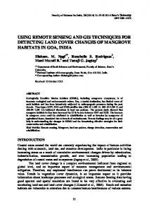
The proposed approach is described in figure 1:
Analysis
Primary Data
Database
Feature Extraction Process Preprocessing
Ortho-rectified images
•
Tax-assessor parcels Parcel geometry Parcel location Tax data attributes
Building Inventory
Parcel-based image partitioning
Initial Analysis • Histogram analysis Analysis, Validation, Elimination • Geometry-based Elimination of low-probability building segments • Use of shadows for building segment verification and elimination Output processing • •
Raster to vector Generalization
Figure 1 – Methodology of the building extraction approach 1.2
Problem Statement This research is primarily aimed at automating the building footprint extraction
process from remotely sensed sources, and as a corollary, minimizing the need for human intervention. The automated extraction process will be based on simple parameters either available or derived from the scene and parcel data, and will not require prior knowledge or expertise in photogrammetry or remote sensing.
The research project will also
evaluate the robustness of several extant techniques for building extraction. The study will also implement the generated techniques by integrating both vector and raster data sets in a new manner, to achieve a more complete and reliable solution.
4
1.3
Significance and contribution to the field
The contribution of the proposed methodology can be evaluated as contribution to the industry and academic research that demands building inventory, contribution to the automated feature extraction effort within the photogrammetry and remote sensing discipline and contribution to both image processing and photogrammetry by introducing image processing techniques rarely used within the remote sensing and photogrammetry field (such as the moment theorem) towards building extraction.
Moreover, the
methodology will attempt to expand work done within image processing and can be used for processes other then building extraction. There is evidence in the literature that supports the need for more research on automated systems for feature extraction that combines geographical information from different sources and uses GIS data as a-priori knowledge (Brenner, 2005; Baltsavias, 2004). The methodology as presented introduces a new overall approach to building footprint extraction. The integration of GIS and remote sensing sources as presented has not been implemented and tested as an entire approach to solving the problem. Simplification algorithms have been evaluated and tested in previous projects. Hence, using parcel geometry and parcel attributes for simplification purposes will extend work done by Wijnant and Steenberghen (2004), Ming et al (2005) and Ohlhof, et al (2004) by evaluating the added value of using readily available parcels layers and attribute information for simplifying the task. The automated building extraction procedure may be developed into additional inventory (roads, sidewalks etc) development tools in GIS and would enhance and benefit 5
a wide variety of applications.
Building locations are required for day to day
management of cities and counties and for more complex applications such as evaluating damage after an earthquake.
All those applications can benefit from a
methodology/automated procedure that can produce a large percentage of the building inventory and hence, maintain an updated inventory.
Brenner (2005) anecdotally
mentions a German city that acquired about 30,000 km² of features. Each building required several points, which required a huge effort. The company estimated that an update of the area will require about 70% of the initial effort. That number emphasized the concept that building extraction does not require only an initial investment, but is an on going expenditure. The photogrammetry and remote sensing field has been attempting to develop automated and semi-automated approaches for feature extraction and in particular building extraction over the last 15-20 years. Today, we still do not have an “accepted” methodology to extract buildings from aerial imagery and therefore we normally digitize those features manually. An automated approach that can be easily replicated and takes advantage of readily available sources may contribute to that effort. The work can be viewed as a direct continuation/expansion of the work by Huertas and Nevatia (1988) that pioneered the usage of geometry and shadows for the purpose of building extraction based on edge detection, and the work of Irvin and McKeown (1989) that used shadows in different stages of the extraction process. The methodology extends many projects that concentrated on extracting specific types of buildings such as Kim et al (2004) that developed a methodology to extract large rectangular buildings. The methodology also expands the approach taken by many research projects that involve semi-automatic tools 6
with more considerable user intervention (especially for simplification), such as Müller and Zaum (2005) that uses seed growing mechanism and Sahar and Krupnik (1999) that initially break the image manually into regions of interest. The methodology is aimed at high-resolution (1ft) imagery that is the current standard for urban aerial imagery and more elaborated than the more heavily tested 1m resolution aerial and satellite (IKONOS) imagery. The work of Hu (1962), Rosin (1999) and Rosin (2003) is used and implemented in the proposed methodology. Although used within the image processing discipline, the moment theorem has not been commonly and heavily applied within the photogrammetry and remote sensing field for building extraction. Evaluation of using this theory for the purpose of identifying building segments can contribute to the long effort of extracting buildings and possibly other types of features. As mentioned above, we attempt to specify index not only for rectangular shapes (Rosin, 2003), but for the “I” and “O” shapes, from the common L, T, C, I, H, O building footprints.
Successful shape
identification extends the work of Rosin (2003), Reiss (1991) and Schweitzer and Straach (1998) that evaluate properties of specific shapes based on moment invariants. 1.4
Organization of Dissertation
This dissertation is organized into six chapters. The introduction chapter describes the need for automated building extraction procedures. The chapter details the problems involving the extraction procedure and the added value of the proposed methodology. The introduction also defines the scope of the dissertation.
7
Chapter 2 reviews the current state of building extraction procedures within the photogrammetry and remote sensing field. The review includes a survey of extraction procedures using different types of imagery, including aerial imagery, satellite imagery, LIDAR, and RADAR.
The review details the different image processing techniques
used for the purpose of feature extraction and building extraction in particular as well as shape recognition techniques using the moment theorem. The chapter also includes the basis for the motivation of incorporating GIS data in the methodology as well as moving from global image processing to a local image processing approach. Chapter 3 presents the current methodology of the project. The chapter illustrates the flow of the building extraction model and provides a general description for each analysis phase. The chapter is followed by a detailed description of the methodology implementation.
The description in chapter 4 includes the tools, algorithms and
techniques used to implement the image partitioning, segmentation, feature analysis and generalization of the buildings outlines. Chapter 4 contains two sections. The first section presents the implementation details and the second section presents and evaluates the results of the testing. The results evaluation section begins with general details about the testing area and the datasets. The general information is followed with a test plan for different types of buildings within the testing area. The testing evaluation includes a discussion of the success or failure and provides further analysis where required. The evaluation includes an in depth analysis of the factors that prevent successful extraction and also recognizes those scenarios that allow automatic extraction of buildings from aerial images.
8
Chapter 5 concludes the document and provides recap of the entire process as well as final remarks from the author regarding the contribution of the project, the recognized limitations for the approach and possible future research.
9
Chapter 2 LITERATURE REVIEW The work presented in this report is mainly concerned with the possible automation of the building extraction procedure.
The research and technological advances in
photogrammetry, remote sensing and computer science introduced a remarkable potential for reducing human involvement in building urban inventory. The methodology tested in this work involves different image processing techniques at different stages and emphasizes the need for data fusion during the extraction procedure. This section begins with a review of the history of photogrammetry and major mile stones that lead to the current digital era. Section 2.2 entails a general review of the building extraction procedure and approaches taken in research for this purpose. Literature for the building extraction procedures is described in section 2.3 as well as image based classification techniques. This section deals mainly with extraction from high resolution imagery.
Section 2.4 elaborates on image processing techniques used
for the extraction of buildings from aerial imagery, including classification methods and shadow extraction. Section 2.5 emphasizes the need to incorporate existing GIS data within the extraction process.
Different approaches that take advantage of existing
spatial information are descried. Section 2.6 provides a short review of LIDAR and laser scan technology. Although not pursued within this project, the unique advantage of this technology for feature extraction is acknowledged.
As an important part of the
methodology of this project, section 2.7 explicates the inherent value of subsetting an image into smaller patches prior to extracting the building. Section 2.8 reviews the moment theory as a tool for shape identification as relates to the methodology.
10
2.1
Evolution of photogrammetry and Remote Sensing leading to feature extraction Photogrammetry has changed dramatically along side the technological advancements
as developed in the past century. The evolution period can be divided into several phases (Konecny, 1985; Madani, 2001).
The first phase is referred to as the “Analog
Photogrammetry”. This phase began around 1900 (Konecny, 2003) and inaugurated the use of aerial imagery for mapping purposes. The mapping process was based on stereoplotters and the “stereoscopic measurement principal” (Konecny, 2003). Stereo plotters reconstruct the relative location and orientation between images at the time they are captured. Due to the different perspective of the images, a 3D model is created for the overlap area between the images. The model was mainly used to capture elevation and contour lines.
The next phase began in the 50’s and is called the “Analytical
photogrammetry”. The analytical photogrammetry introduced the first aero-triangulation implementation, DEM generation and feature extraction as a result of the breakthrough of computer-aided techniques and applications in the 60’s (Madani, 2001). The third phase is the computer-aided phase that started in the early 70’s and introduced a new level of efficiency to the mapping process. During this phase we see the emerging computer and graphic processing abilities (such as CAD systems) as they become more and more dominant in the photogrammetry arena.
The last and current phase is the “Digital photogrammetry”. The inherent difference between that phase and the previous phases lies within the nature of the imagery. The digital era deals with pixel image coordinates and grey levels, while previously the hard 11
copy image was the input media. The greater power of computers and workstations, satellite imagery, photogrammetric cameras (including CCD, line scanners), on board GPS systems, scanners, RADAR technology have made an impact. Currently even personal computers are able to perform many tasks that require massive processing power and space.
Advances in computer science and implementation of photogrammetric
principles and techniques such as AeroTriangulation, orthophoto and DTM generation, allowed the photogrammetry and remote sensing community to move in a new innovative research path towards automation of more complex procedures. Tasks such as feature extraction are still in research as they were in the last three decades.
There is a
fundamental agreement that photogrammetry and remote sensing can provide an efficient and relatively easy way to collect data and maintain updated GIS systems for purposes such as resource management. As imagery improves in spatial and spectral resolution and becomes more available, we are able to extract better, more accurate information. Still today, many processes rely on a human interpreter to distinguish between different features and digitize the accurate positions of objects. 2.2
Building Extraction – General Many studies presenting automatic or semi-automatic approaches to building
detection have been published. Building extraction poses several major difficulties that any system has to overcome (as discussed in section 1.1). Marr (1982) describes the human vision as an information-processing task. This task encompasses many aspects of a human perception, such as shape, space, spatial arrangement, illumination, shading and reflectance.
Since we can not fully imitate the human brain functionality, it is a
challenging task to automate image vision and interpretation. Hence, operators are still 12
indispensable during the feature extraction phase, and many applications use a semiautomatic approach to extract point, lines, areas and complex objects (Vosselman, 1998). This approach utilizes the advantages of the human as well as the superiority of the computer for specific, repetitive tasks. Line following mechanisms, based on an initial point on the road, have been prominent for road extraction (Aviad and Carnine, 1988; Gruen and Li, 1995). Similarly, the user may specify the approximate location of an object and the computer will then perform a specific task such as a seed-growth algorithm (user defined starting point and growth according to value similarity between pixels) to locate the boundaries. Alternatively, users may locate one corner and using edge detection to locate the rest, acquiring approximate location of the corners and having the computer snap to the nearest “point-of interest” (the corner). A third approach could employ manual digitizing in one image and using epi-polar geometry between the stereo pair to locate the height and the corresponding points in the second image (Tao and Chapman, 1997). The extraction of areas (polygons) is based on homogenous surface attributes such as grey levels (similar color for water areas, roof tops etc.). One drawback of implementing that approach on an entire image is the wide variety of grey levels within the group of man-made buildings. 3D objects such as buildings are mostly referred to in the literature as complex objects. For the extraction of those objects, the user utilizes geometric constraints to extract linear parallel lines for building edges and match those edges to overlapping images.
Man made feature extraction process can take advantage of
supplementary information such as DTMs (Digital Terrain Model) for both building and road extraction. That information can be used to impose geometric known characteristics 13
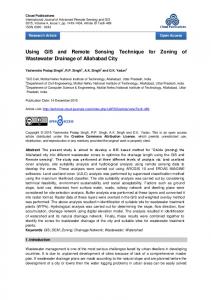
such as moderate changes in height along a road or a river, or rectangularity of buildings. These constraints can make the extraction process much more robust and reliable. Figure 2 portraits the main approaches, techniques and sources of data for building extraction, as described in the given research review.
2D Extraction Mono (1 image) Aerial Photo Satellite Image
Seed Growing Edge Detection & line Segmentation Geometric constraints Clustering Other Image processing Techniques Supplementary GIS data
3D Reconstruction
Shape Recognition
Stereo Imagery Shadows
Image matching techniques Shadows extraction
Point to Surface conversion Bare earth extraction Feature extraction
LIDAR
Figure 2 – Main Approaches to Building Extraction
Aerial Photographs and high resolution satellite imagery are the most common sources of data for feature extraction. In order to extract 2D characteristics of a feature, a mono image may suffice. 3D features such as buildings often require analysis of 3D cues (such as shadows) within the image in order to adequately detect and extract the outline. Any 3D reconstruction of the feature requires either stereo imagery (two or more images with enough overlap area) or sophisticated extraction and analysis of shadows cast by the features. 14
2.3
High Resolution Satellite Imagery
2.3.1
Data Classification Techniques from remotely sensed data
Image segmentation and classification is a common and prominent method for extracting information from images in many disciplines, using a wide variety of well established approaches as well as new, innovative techniques (Wang et al, 2001; Bin et al, 2002; Chen and Wang, 2004; Zhang et al, 2006; Zebedin et al, 2006). Segmentation is usually a first step in a process followed by subsequent analysis of the features and possible object matching algorithms. The computer science community has shown great interest in image segmentation, much of that for the purpose of image retrieval from a database (Ahu and Yuille, 1996; Shi and Malik, 2000). Smeulders et al (2000) discusses the difficulty of reaching a “strong” segmentation. He then continues to discuss “weak” segmentations that result in homogeneous regions within the image that do not necessarily cover entire objects. Compromising for a “weak segmentation” gives a rise to numerous problems in the following steps of the process and to the overall success of the image interpretation. Classification of data from aerial and satellite imagery is a well known approach within the photogrammetry and remote sensing communities. Remote sensed data enabled a replacement of in-situ measurement for disciplines such as forest management. Information that is otherwise very hard to obtain, is available through images for planners, ecology modeling, and many other disciplines (Jensen, 2005). The remote sensing data collection records the amount of radiation reflected by the object, thus creating a “signature” of the object. The signature of the objects holds much information
15
about the characteristics of the objects. We are able to classify different types of objects and even sub-object using classification methods.
Remotely sensed data is usually classified using methods that can be categorized as: Supervised and Un-Supervised classification. A Classification is mainly an automatic or semi-automatic way to identify the signature of each class and their location in the image. The final goal of the classification is usually to yield land cover/ land use classes for the area of interest. Supervised classification – supervised classification assumes prior knowledge through personal experience, interpretation of aerial images and map analysis (Jensen, 2005; Hodgson et al, 2003). The analyst manually trains the system by locating areas in the images that comprise of the classes of interest. The user should strive to define distinct classes with the least amount of overlap between them (in the spectral space) in order to allow better classification. To that goal, the user may take advantage of spectral plots that easily portray the degree of correlation between the classes. For each class, the system calculates statistical measures (Standard Deviation, Mean, covariance matrices etc). During the classification process, every pixel is assigned a class according to the highest likelihood of being a member of the class. Once the classification is complete, a rigorous error evaluation takes place and statistics are available to the user. There are different types of algorithms that can be used for the classification. Those can be divided into parametric and non-parametric classifiers. The parametric assumes normal (Gaussian) distribution for the observations (Schowengerdt, 1997). The most 16
common supervised classification method is the maximum likelihood algorithm (Ozesmi and Bauer, 2002; McIver and Friedl, 2002). This classifier calculates a probability density function based on statistical measures of each class. By placing the brightness value of the pixel in the probability function, we obtain the probability of the pixel being a member in a class. The pixel will be assigned the highest probability class. The most common non-parametric classification algorithms and techniques are (Jensen, 2005): Parallelepiped – Parallelepiped classification is a fairly simple to implement and efficient algorithm. For each band and class, the algorithm calculates the mean and standard deviation values. The result is an n-dimensional vector with all the mean values of the trained data for each class in each band. The boundaries for each parallelepiped are defied based on 1 standard deviation values.
A pixel is evaluated according to the
high and low standard deviation values (greater then the lower boundary, less then the high boundary) and if not suitable to any class, it will be assigned to an unclassified class. A problem may occur when parallelepipes overlap. In such cases, the pixel is usually assigned to the first found class or a criteria rule such as minimum distance can be used to make the decision. Minimum distance(MD) – Similar to the Parallelepiped algorithm, the minimum distance algorithm first calculates the mean values for each class in each band. The result is a mean value vector for all the trained data. During the classification, the algorithm performs distance calculation between each pixel and the mean vectors. The minimum
17
distance determines the class assignment. The user is given the option of defining a maximum distance that beyond, the pixel will not be classified. Nearest neighbor (NN) – The simplest non-parametric decision rule that weighs nearby evidence more heavily, thus classifies a pixel to the nearest class (Cover and Hart, 1967). The calculated distance between the pixel and every class is Euclidean distance. Other, less simple algorithms such as the k-nearest neighbor search for the closest k number of training pixels in the feature space to determine the class. Artificial Neural Networks (ANN) – Neural networks have been increasingly applied within numerous applications over the past decade (StatSoft, 2003; Makhfi, 2007). The ability of ANNs to learn and reach a decision, like a human, has captured the interest of researchers from many fields. ANNs have been used to make prediction such as future stock performance (Makhfi, 2007), data modeling, function regression, pattern recognition (California Scientific, 2007) and more. The concept of neural networks was first introduced by McCulloch and Pitts (1943), but required the advancement of computer technology to be successfully developed and applied. ANNs simulate decision making processes as achieved by inter-connecting neurons in the human brain (Jensen et al, 1999). The decision making process is based on initial training of the network. Input and desired output examples are provided to the network.
During the learning process, the weights of the different connections are
adjusted to achieve the specified outputs. There are two main advantages that made ANNs appeal to the remote sensing community: ANNs do not require a normal distribution (hence, it is not necessarily a 18
parametric classifier) and they can simulate non-linear patterns (Jarvis and Stuart, 1996; Jensen et al, 1999; Jensen 2005). ANN has been implemented in remote sensing software such as ENVI, but there is no clear consensus about the superiority of ANNs over traditional classifiers.
Several projects demonstrated better classification results for
ANNs (Ji, 2000; Bischof et al, 1992; Jensen et al, 1999) while others show no significant advantage to ANNs or expressed more caution (Hepner at al, 1990; Jarvis and Stuart, 1996). Moreover, since there is no clear explanation to the rules as created by the neural network, it is being assessed as a “black box” (Qui and Jensen, 2004). Hence, users are reluctant to use those systems for real world scenarios. Another major disadvantage of ANNs is the training process that requires the users to be very knowledgeable about both neural networks and the area of interest for the classification.
This is a major
disadvantage due to the relative simplicity of running any other traditional classification. Unsupervised classification - Unlike Supervised classification, Un-supervised classification does not require prior knowledge about the area of interest, thus, no training is required. The system searches for natural grouping/clusters of the pixels (Jensen, 2005). The most commonly used classification methods are the ISODATA and K-means. ISODATA - ISODATA stands for Iterative Self-Organizing Data Analysis Techniques (Ball and Hall, 1967). No prior training is required, but the algorithm needs a starting point and thresholds (Fromm and Northouse, 1967) for split, merge and stop criteria. The algorithm assumes Gaussian distribution of the pixels in each class. The criteria parameters include (Jensen, 2005) the maximum number of clusters; the maximum percentage of pixels allowed being unchanged between iterations - when the system reaches that number, the process stops; Maximum number of iterations - each 19
iteration involves recalculation of the class mean and re-reclassification of pixels; Minimum number of pixels in a class; maximum standard deviation for a class; minimum distance between cluster means; Split separation – if not 0, this value will be used to decide on the location of the new class when splitting large classes rather then using the standard deviation. The algorithm begin by calculating initial mean vector for the classes, and iteratively move pixels between classes, merge classes or split classes based on the input parameters. The ISODATA algorithm is considered slow (Jensen, 2005). K-means – The goal of the k-means algorithm is to divide pixels between clusters in a way that the sum of squares within each cluster is minimized (Hartigan and Wong, 1979). The mean position of all pixels within a class defined the center of the class. Pixels move between classes based on the Euclidean distance to the center of the class. Sometimes, the boundaries of phenomena may not be distinct, but rather fuzzy. In the image space, a pixel may contain more then one land cover class (“mixed pixel”). In order to handle this case, a fuzzy classification algorithm may be used instead of the hard classification methods described above (Laha et al, 2006). A fuzzy algorithm is based on replacing the hard boundary between the classes with more gradual transition between the classes. Those methods assign to each value several probabilities according to the set of classes it might belong to (Jensen, 2005). In the past decade we have witnessed the development of object-oriented classification methods. Unlike the per-pixel classification algorithms, Object Oriented classification techniques aim to extract homogeneous regions within the image that bear
20
meaningful information. The image is usually divided into sub-areas based on spectral and spatial characteristics and then each region is assigned to a class (Wang et al, 2004). The combination of spectral and spatial information is useful for land cover classification since, often, the same class encompasses several similar spectral signatures or different classes share spectral signatures. The classification techniques illustrated above have been widely employed by the photogrammetry and remote sensing communities for land cover classification. The classification processes were based on one specific technique (Samaniego et al, 2008; Davis and Wang, 2002) or a fusion of several algorithms. Zebedin et al (2006) illustrate an approach to automatically generate land cover/land use maps from aerial imagery. The images include both high resolution series of panchromatic overlapped images and low resolution multispectral images.
The methodology encompasses different
classifications – maximum likelihood, neural network, decision tree and support vector machine. Substantial effort is devoted to image matching DTM and DSM (Digital Surface Model) generation and AT (Aerial Triangulation). Their result is a raster land cover classification map that showed a high accuracy of vegetation detection. Li, Wang and Ding (2006) propose a feature extraction method that can be used for urban area mapping based on a potential function clustering method.
This clustering method
segments the image by selecting peaks within the image histogram. The claim is made that, within an urban image, a grey level histogram peak can be used to segment the entire image. Once the segmentation is complete, the buildings can be selected manually. Every candidate is extracted using seed region growing followed by edge detection, dominant line detection and outline mapping. The method was tested on a region within 21
a Quickbird image (0.61m) that, based on the example provided, includes mostly regular buildings. The results shown were visual and the accuracy was depended on the selected grid size for the building outline mapping.
Segmentation is an early step within the building extraction process in this project. By analyzing the histogram of a localized image, regions in the image are segmented and analyzed to identify buildings. This approach can be more closely related to the objectoriented segmentation approaches as discussed above. 2.3.2
Building Extraction from Satellite Imagery
Fraser et al (2002) investigated to ability to extract buildings manually from IKONOS imagery in order to construct 3D models. One of their conclusions was that about 15% of the buildings could not be identified in the imagery. They reported possible sub-meter accuracy for stereo input images under certain conditions and data configuration. Xiao, Lim, Tan and Tay (2004) use high-resolution IKONOS satellite stereo-pairs to extract roads and 3D models of buildings. The building extraction relies on existing roads and previously extracted vegetated areas. The building extraction process is semi-automatic, based on edge detection and “thinning” and allows the user to select between several potential rooftop alternatives and adjusts corners and edges. For small buildings, the user may predefine rooftops to be recognized using Neural Networks. Heights are eventually computed using the stereo-pair images.
Sohn, Park, Kim and
Heo (2005) propose a building extraction method based on high resolution IKONOS multispectral stereo pair images.
The algorithm is based on an image processing 22
technique BDT (Background Discriminant Transformation) on multi-spectral images. This technique is scale invariant, reduces the variability in the background, and enhances the non-background. Similar to the principal component, several bands are created with maximum to minimum differences between the background and the non-background (here, the potential feature). The result of the first step allows the classification and clustering of buildings. Once the buildings are enhanced using the previous step, they are clustered by the ISODATA algorithm (See section 2.3.1). In the next step, using color indexing and distance measurements, matched buildings between different images are located. Matching the buildings between the stereo-pair enables the generation of a 3D model. This article highlights the growing need for extracting 3D characteristics of objects. This is definitely an open problem that needs to be tackled, although the results reported emphasize the need for future research that could utilize information such as shadows, since matches failed mostly owing to buildings obscured by shadows. Wei, Zhao and Song (2004) use image processing techniques in order to extract buildings from high-resolution satellite imagery (using Quick Bird panchromatic images). Their application is based on unsupervised clustering using histogram analysis and shadows in order to detect and locate buildings.
Edge detection and subsequent Hough
transformations are used to extract the dominant lines of the buildings and construct the building footprint.
23
Table 1 - Sample of available aerial and satellite imagery
Sensor Type
Spatial Resolution
Radiometric Resolution
*Panchromatic 0.5 ft 212 (0 - 4096) *Color film 0.5 ft 212 (0 - 4096) *Color IR film 0.5 ft 212 (0 - 4096) *Panchromatic 1 ft 212 (0 - 4096) *Color film 1 ft 212 (0 - 4096) *Color IR film 1 ft 212 (0 - 4096) QuickBird-2 Pan 0.6 m 211 (0 - 2048) QuickBird-2 MSS 2.4 m 211 (0 - 2048) IKONOS-2 Pan 1m 211 (0 - 2048) IKONOS-2 2.4 m 211 (0 - 2048) IKONOS-2 MSS 4m 211 (0 - 2048) SPOT-5 Pan 2.5 m 28 (0 - 255) SPOT-4 MSS 20 m 28 (0 - 255) SPOT-1,2,3 Pan 10 m 28 (0 - 255) SPOT-1,2,3 MSS 20 m 28 (0 - 255) Landsat TM 7 Pan 15 m 28 (0 - 255) Landsat TM 7 30 m 28 (0 - 255) * - spatial resolution depends on sensor altitude
Temporal Resolution
Varies Varies Varies Varies Varies Varies 3 days 3 days 3 days 3 days 3 days 3 days 3 days 3 days 3 days 16 days 16 days
For testing the methodology presented in this research, we will use 1ft resolution color aerial imagery. That detailed resolution allows an accurate detection of the building outline. At the same time, this resolution presents problems such as the inability to use simple clustering functions (such as ISODATA) that are common for coarser resolutions (See SPOT and Landsat in table 1).
24
2.4
Image processing techniques According to pre-defined models of buildings, Huertas and Nevatia (1988) impose
geometric constraints during the detection stage, and shadows are used to verify the outline of the feature as well as to estimate the height. Shadows have been used in different stages of extraction by Irvin and McKeown (1989), as part of shape prediction, grouping, verification and height estimation. Constraints are the core of the building recognition proposed by Kolhe, Plumer and Cremers (2000). Their approach is based on constraints and logic programming, and employs hierarchical building models with 2D and 3D representations. Sahar and Krupnik (1999) used methods that combine edge data, stereo-analysis and shadows in order to extract the 3D shape of the building.
3D
information was found to be a significant source of information for the building detection process. Sung Chun, et al (2006) developed a system aimed at 3D extraction of the building outline. The user selects a point within the building on one image and the system locates the matching feature on other images and provides the best 3D hypothesis for the building. The experiment results show an efficient semiautomatic approach for 3D complex buildings. Weidner and Förstner (1995) generate a high-resolution DTM, and with topographic data available for the scene, they extract and reconstruct the buildings. Shi and Shibasaki (1996) use stereo imagery and line-based matching to overcome the absence of shadow information in an image in order to estimate ground elevation and evaluate the 3D lines of the building. Avrahami et al (2008) describe a method to extract rooftops based on the assumption that rooftops are combination of polygons. The approach consists of both manual and automatic steps, where the user has to select a parameterized model for the extraction and point to the location within the left
25
image. Based on that input and the right image, the roof is constructed. Multiple building extraction procedures were developed to identify buildings from a single image (mono). Kim et al (2004) developed a methodology to extract large rectangular buildings from 1m resolution imagery using a single image and line detection techniques.
The
user’s interaction includes clicking on a point inside the building, and initiates a seed location for the process to identify the boundaries. Their results conclude that short sides of the buildings are not well extracted and there were several cases of false line extraction. Although some buildings were not oriented correctly, they believe the overall approach of pointing the building as a cue is a promising approach. Müller and Zaum (2005) present an approach based only on an aerial image and image processing techniques. Their approach initially uses a seeded region growing mechanism to segment the image.
Segments are then evaluated using geometric (area, roundeness etc)
photomentic (Hue angle, mean hue angle etc) and structural (Shadows, relationship to other extracted buildings etc) parameters.
Jin and Davis (2004) integrate different
algorithms based on spectral, structural and contextual (position and size of adjacent buildings) information in the image. Their approach is aimed at 1m IKONOS imagery and they develop a DMP (Differential Morphological Profile) to generate the structural information as well as extract shadow regions. The evaluation report shows that 72.7% of the building areas are extracted with a quality percentage 58.8%.
Over 70% is
considered a good success rate, while the 58% quality shows need for improvement. Some gabled roofs and dark parking lots were not detected or falsely classified as buildings. Lee et al (2003) used supervised and unsupervised classification techniques on both the multispectral and the panchromatic images of IKONOS satellite. Their building
26
squaring techniques were based on Hough transformation and their overall extraction rate is 64.4%. Most misclassification occurred owing to shadow inclusions and false road classification. Tang et al (2004) tackled the problem of extracting high rise buildings. High-rise buildings usually have complex shapes and have not received enough attention within the feature extraction research.
The extraction procedure was based on
identification of vertical lines in a mono image using fuzzy Hough–transform, complemented by photogrammetric principles that provide clues about the location of vertical lines in the image. Locally, the authors analyze the texture of the windows on the wall of the building. Roof extraction was accomplished using edge detection and line segmentation. The approach was tested on a 0.2 meter scene from an aerial image and reconstruction results were presented for four high rise buildings in the image. The methodology of this research is geared towards minimizing user’s intervention; therefore, techniques such as selection of a starting point for seed growing, is not used. Shadows are extracted as means of verifying the location of the building and eliminating non-building (2D) features. The process also evaluates the geometry of the feature as well as the validity of the building candidate based on geometric characteristics such as minimum size and width. 2.5
Supplementing with existing spatial data Existing GIS data provides prior knowledge about the area and can add considerable
value to the extraction procedure. Baltsavias (2004) provides an overview of the status of feature extraction in research. The author acknowledges the need for more projects that exploit a-priori information.
He points out to the fact that only few use a-priori
knowledge in the form of GIS data, maps and geodatabases. Duan, Prinet and Lu (2004) 27
used GIS data about the position and shape of buildings. Their application uses a fuzzy segmentation technique for roof extraction without allocating the actual footprint of the building.
Segmentation of the building area is accomplished using seed growing
mechanism. The seed point is selected by calculating centroid points for buildings in a GIS building layer.
The building vector layer is converted to a raster image. The
segmented regions and the original building raster image are compared through out the process to minimize differences in area between the polygons. Koc and Turker (2005) developed similar applications to update an existing vector building layer. They utilized image Supervised classification, NDVI (Normalized Difference Vegetation Index – indicator of vegetation presence in remote sensing images), DSM (Digital Surface Model) extracted from a stereo pair and object extraction techniques.
Khoshelham
(2004), demonstrate the fusion of images data, height and plan 2D data (XY coordinates of the roof) to reconstruct the 3D model of the building. The images used in that project include the near IR channel and hence allow simple identification of vegetation for the first step of vegetated-area elimination. Available GIS data such as tax assessor attribute data is used in this research as a cue for existing buildings, as well as a way to eliminate different areas within the image. For example, vacant parcels are not searched. In vegetated area, NDVI can be used as a first step of pre-processing before running the proposed application. 2.6
LIDAR and Laser Scan based methods In recent years, LIDAR points have become a valuable source of data for feature
extraction. The density of the points allow the generation of detailed DTMs as well as extraction of buildings, roads and other features (Gamba and Houshmand 2000, 28
Rottensteiner, Trinder and Code 2005, Nardinocchi, Scaioni and Forlani 2001). Rottensteiner, Trinder and Code (2005), describe their effort in automatic extraction of buildings and roads using LIDAR data. Current LIDAR resolution, while high (about 2m), actually causes ambiguity between buildings and vegetation features such as trees for the extraction process. Overcoming that ambiguity requires the use of other sources of information such as intensity and/or RGB orthophoto that allows the classification and subsequent elimination of vegetation using NDVI or pseudo-NDVI.
In the project
described in the article, a 2 phase algorithm was developed in which the buildings are first detected and then reconstructed.
The detection is based on a pixel-based
classification. The authors defined 4 basic classes - buildings, trees, grass and bare soil. Each pixel receives a probability score of being in each class (sum of all probabilities for each pixel is 1). Other measures are used to eliminate different classes. For instance, differences in height between the DSM and DTM can distinguish between building/tree object groups and flat grass/bare earth object groups. Vegetation indices can distinguish between tree/grass object groups and building/soil groups. By imposing these tests, a binary image is created where buildings are high-lighted.
The result is refined by
eliminating areas that are suspected as trees. The method failed mostly in residential small buildings and using NDVI seemed to increase the accuracy and extraction results. (95% of all buildings greater than 40 sq-m; buildings smaller a 30 sq-m were not detected at all). Finally, the reconstruction of the building and extraction of the boundary is created with the aid of GIS external data (such as streets to separate buildings) and geometric characteristics for buildings.
Sohn and Dowman (2003) presented their
approach to building extraction that includes a recursive extraction procedure to evaluate
29
the existence of buildings within both the LIDAR cloud and IKONOS image. The building extraction was achieved using hierarchical segmentation of LIDAR DTM complemented by color imagery. Building detection using LIDAR point data is currently beyond the scope of the research, mainly since LIDAR data are not widely available for every urban area. Future research can investigate the integration of the proposed approach with available LIDAR data.
30
2.7
Image subsetting approaches
Image partitioning has been tackled within the computer science community mainly for the purpose of content-based image retrieval and matching. In order to effectively retrieve information automatically from images, global image analysis is rarely sufficient. Numerous algorithms have been developed to partition the image into regions that allow easier interpretation of the objects (Berretti et al, 2000; Carson et al, 2002; Yixin and Wang, 2002; Jia and Wang, 2003; Chen and Wang, 2004). The regions are created either by subdividing the image into pre-defined region sizes or number of regions, or locating homogenous regions in the image. The inherent problem of pre-defined subdivision of the image is the cutting of objects between regions. Jiang, et al (2008) provide a semiautomatic methodology that first partition the image into homogeneous regions via image segmentation. The segmented regions are then processed to improve the segmentation result. The building extraction is performed within the homogeneous regions through an interactive selection of points for seed growing and then a region merge to union the buildings and remove overlaps. Finally, edge detection is performed.
The method was tested on RGB image with 20cm
resolution on an area that spans 867×617 pixels that consists mostly of regular buildings. The result was compared with ISODATA classification result. Zhengjun, et al (2008) present a region based and feature based methodologies for building extraction. The region based method relies on localized region extraction.
In order to extract
homogeneous building regions, the user manually identifies an area that contains buildings and background. This area is used to launch a mean shift segmentation method 31
that results in the areas of attraction. A seed growing technique based on manually selecting the area of the building is applied on the segmented result. Boundary fitting and shape recognition follow that step. The feature extraction methodology is based on edge detection (Canny), line and corners detection followed by locating the boundary of the building and shape reconstruction. Constraints on the length and the right angle search process for the corners are imposed. The methodology was tested on QuickBird imagery and shows success rate of 75% (total of 35 buildings were tested) for extracting major rectangular and regular building rooftops. Sohn and Dowman (2003) simplified the building extraction procedure in an urban scene by localizing the search to the building area. Their approach was based on LIDAR points and a technique that automatically distinguished between on and off terrain points. In order to differentiate between those types of points, the technique located homogenous slope sub regions in the LIDAR point cloud. This localization approach failed for most residential buildings. The low density of LIDAR points and surrounding trees seemed to be the leading reasons to the failure. As regions as sub areas in the image are discussed within the computer science discipline, parcels as sub areas are commonly discussed within the GIS community. The next several articles have a title that incorporates the term “parcel” for feature extraction. Wijnant and Steenberghen (2004) used parcels as a measure to summarize land cover classes for land use rather then to reduce signature confusion. Their methodology includes initial per-pixel classification of the 1m image to acquire land cover classes and then summation of the classes per parcel to distinguish different land use parcels by the type of classes they contain. Ming et al (2005), use the term parcel as related to a region or a field that is acquired by initially breaking the image 32
into homogeneous segments based on computational rules. A significant aspect of their project is developing a mechanism to partition the image based on spectral, texture and relationships between objects at different scales. Partitioning of the image occurs from rough classification on a large scale to more focused processing on the more elaborated and smaller regions. One of the major conclusions of the paper is the necessity to break the image into smaller areas.
Ohlhof, et al (2004), also refer to parcels as regions that
have statistical parameters that differ from their neighbors, are homogeneous and have distinct boundaries. Their projects involved development of an algorithm to extract those regions from the image as well as region growing techniques based on geometric and radiometric characteristics of the features. An easy way to partition the image prior to the building extraction process can tremendously simplify the entire procedure. In this research I suggest the use of a graphic parcel layer to restrict the search to the close proximity of the building. Each parcel is cut through the image to create a smaller search region that contains one or more buildings. 2.8
Shape identification techniques and measures The different candidates for the features are segmented in the image space.
A
significant problem is first to be able to describe automatically the properties of the segments. Delineating segment properties allow the evaluation of the probability of a segment to be part of a valid feature. Prokop and Reeves (1992) provide a significant survey of techniques based on moments for the recognition and representation of objects. The survey includes different types of moment invariants, the image ellipse and a variety of applications that take advantage of the “moment theorem”. Hu (1962) introduced the 33
use of image moments for pattern recognition. In this ground breaking paper, Hu showed the ability to determine the shape of a pattern using moment invariants. Hu introduced seven different moments that define the area, COM (Center Of Mass), orientation, elongation in both axes (the standard deviation ellipse). Higher order moments can be defined to be invariant to scale, skewness and rotation. Hu showed that using moments can distinguish between letters of the alphabet. Using the first two invariant moments, Hu defined X and Y coordinates and plotted them on a simple 2D Cartesian coordinate system. The result plot demonstrated the distinct separation of alphabet characters over a graph. A new letter can be identified by the minimum distance to an existing point on the graph.
Alt (1962) used moments to show that a limited number of moments are
sufficient to describe and distinguish between patterns such as letters and numbers. Reiss (1991) claims to discover mistakes in Hu’s theorem and revised Hu’s moment to be invariant under general linear transformations as well as changes in illumination. Reiss also laid a foundation to evaluation of specific shape quality by calculating invariants specific to square and equilateral triangle shapes.
Schweitzer and Straach (1998)
expanded the moment invariant theorem to describe automatically the properties of specific shapes based on the identification of the invariant properties of each shape. Their prototype shapes included square, rectangle, right triangle and triangle. Rosin (1999) developed three rectangularity measures, based on MBR (Minimum Bounding Rectangle) and image moments. Rosin showed how using simple algebraic calculation of moments can identify the rectangularity and orientation of the shape in the image. Rosin (2003) expanded his methodology to evaluate ellipticity, rectangularity, and triangularity. Rosin includes measure of circularity, compactness, convexity and eccentricity and
34
shows limited results for automatic identification of all shapes. The best achieved results were shown for a combination of measuring ellipticity using DFT (Discrete Fourier Transform) and triangularity via moment invariants. Elad et al (2004) propose the use of complex moments for reconstruction of planar polygon. This “shape-from-moment” approach extended previous work by calculating moments that are contaminated by noise (which is the expected scenario when working with real world data). Guienko and Doytsher (2003) use moments to evaluate the geometric parameters of features such as buildings and parcels and after training the system, classification rules are used to extract different features within the urban environment.
The “moment theorem” is used in the proposed methodology to evaluate geometric characteristics of each building candidate. Once an area is segmented as a possible building, the raster image is used to calculate the different moments of the segment and as a result evaluate characteristics such as the rectangularity of the feature.
35
Chapter 3 METHODOLOGY The different research projects described above demonstrate several aspects of the extraction process that should be taken into consideration:
Buildings are complex
features and no single geometry can describe them; Edge detection and line segmentation cannot be used as a stand alone solution for the extraction process; The image should be partitioned in a way that will simplify the extraction procedure; Ancillary information, such as GIS data, should be used to complement the solution; Extraction of 3D features should integrate depth cues such as shadows or stereo imagery; Defining segment properties and shape identification measures are essential for the elimination and validation of the extracted segments and hence should be incorporated in the process. Based on the above conclusions and initial experiment results (Appendix I), a methodology based on integrating remote sensing sources and available GIS data is proposed. The remote sensing data sets include high-resolution (1ft) ortho-rectified aerial imagery. Available GIS data sets are used in different stages of the analysis, for initial simplification and filtering and later as elimination, validation and supporting a-priori information for the process. Since buildings may appear in an image (also between images and different resolutions) in a wide variety of shapes and spectral signatures, the proposed procedure refrains from supervised training of the system. Moreover, even though we evaluate the rectangularity of the segments, a rectangle shape is not enforced on the extracted segment.
36
The suggested integration of several GIS sources, their attributes, topological relationships between raster extracted segments and existing vector data, as well as simplification first step based on tax assessor information, form a new, innovative approach for automatic building extraction. Fusion of available data sources with spatial analysis and image processing techniques will provide a robust approach towards solving the problem. The research presents an approach that includes several new approaches to alleviate the complexity of the problem, such as, cutting to parcel size to simplify the image, adding assessor attribute data and including user-one-time-intervention for shadow direction definition.
All the stages, the suggested input information and the techniques are elaborated later in this section with initial experiments results. The steps are depicted in figure 3 below.
37
(1)
Parcel-based image partitioning. Eliminate vacant parcels. Identify parcel type.
(2)
Histogram Analysis
(3)
Feature segmentation in the im image space.
(4)
Parcel-attribute based elimination.
(5)
Use of shadows for building segment verification and elimination
(6)
Geometry-based Elimination of low-probability building segments
(7)
(8)
Fi Finding the footprint: Raster To Vector
Footprint Ge Generalization
Figure 3-Proposed Feature Extraction Methodology
The extraction was based on prior GIS data that restrict the searching area within the scene, and image processing techniques for the extraction.
The following sections
describe the various steps depicted in the methodology flow of figure 3.
38
Parcel-based image partitioning - This first stage can be explained as a simple “cookie-cutting” of the original image into parcel-sized images (referred to as “patches”). Tax assessor data sets that include parcel information are easily available for most areas within the USA and many countries around the world. Moreover, each parcel includes attributes that classify the use of the building within the parcel, whether industrial, residential etc, and specify ancillary information such as built square-footage for taxation purposes. The parcel attribute information can be used to: •
Eliminate vacant parcel (Where improvement value is 0)
•
Distinguish between types of parcels, hence types of buildings.
The extraction
methodology assigns different characteristics to Single Family residential houses and commercial or other types of buildings. Landuse information about the parcel can be used to retrieve the type of building and assist during the extraction. Buildings within the same type are not necessarily within a continuous geographic area. The process, regardless of the location, retrieves the parcel based on the defined type. •
Calculate expected building footprint size – using the square footage and number of stories of the built features (if available).
Zoning ordinance information about each parcel may be used to isolate the area of the parcel, most likely to contain the building. Zoning information provides setbacks for the parcels which define the area allowable for building. Final results of the process may be further evaluated using the zoning information to estimate the added value of zoning for future use within the building extraction process. 39
3.1
Histogram Analysis The histogram analysis is based on locating peaks within the histogram. Peaks in the
histogram represent dominant features within the parcel. Since the parcel is a finite 2D space with limited number of features, the building spans over a significant number of pixels – essentially a peak within all 3 bands (see figure 4).
Investigation of some
preliminary images shows consistent peak generation histogram for the building roof. Within a large sample of buildings in the test images, it was noted that about 50% of the parcels contain a building that creates the majority peak (a highest peak in the histogram). In other cases (see figure 5), the building generates a peak, but not the majority one, and in some cases (figure 6), there is more than one building in the parcel. Within the scope of the project, it will be evaluated whether more then 2 peaks need to be identified in the analytical process.
Band1
Band2
Band3
Figure 4 - Bands 1/2/3 for the image on the left. The high sine wave represents the building. Values span (dark)0-255 (light).
40
Figure 5 - A parcel with a building peak that is not the majority. Zero values are ignored.
Figure 6 - A parcel with two buildings with different roof signatures. Note that the higher peak also includes the parking lot area within the parcel.
41
3.2
Feature Segmentation According to the located peaks within the histogram, features corresponding to the
peaks are segmented in the image space. The segments are then processed further for smoothing and eliminating holes if possible. Currently, results evaluate the usage of only the first and possible second highest peaks for the parcel.
A result of the initial
segmentation is shown in figure 7.
Figure 7 - Preliminary results - Original building on the left; segmented feature of only the majority peak on the right
When different peaks are classified into the image patches, several features are segmented, as shown in figure 8, and the system has to evaluate automatically which segment/s is part of the building.
42
Figure 8 - Segmentation result of 2 peaks within histogram.
Stages 4-6 are used as a mechanism to evaluate whether a segment is part of a building. Segments that are definitely not buildings, based on the different measures, will be eliminated. For the rest, a probability score is attached to each segment at the end as an evaluation measure for the user. 43
3.3
Parcel-attribute based elimination Size limitation may be used to eliminate segments that do not comply with the parcel
built features. The size limitation is either evaluated using the SQUARE_FT and NUM_STORIES retrieved from the attribute table, or calculated as a minimum percentage of the parcel size. 3.4
Shadows Different research projects concluded the importance of using and extracting depth
cues for detection of 3D features such as buildings. Shadows have been proven to be a way to identify the existence of buildings and to distinguish between buildings from flat, ground surface features. For the purpose of this research the user is required to provide simple indication of the sun illumination. A brief look at the image, by any parametric user, can derive that information. A GUI with directions and attached radio buttons can allow the user to define sun illumination aspect as a parameter for the application:
Figure 9 – User GUI for inserting Sun-illumination direction
For Example, in the image shown in figure 10, the user will indicate the 6st (West to East) and 2nd (South and North) radio buttons.
44
Figure 10 - Sun illumination orientation S->N and W-E
Knowing the general orientation of the sun can help distinguish between segments that have the shadow on the correct position related to the segment and are buildings, to non-buildings as can be easily detected in figure 11 below.
Figure 11 - White and Grey segments (right image) share a shadow. The known orientation of the shadow can easily eliminate the grey segment from being a candidate building.
45
3.5
Geometry based elimination of low-probability building segments In this step, the different Hu moments (Hu, 1962) will be evaluated and used for
elimination of shapes as well as other recognized geometric characteristics. Currently in the literature, measures of circularity (not relevant for that procedure) rectangularity and ellipticity (Rosin, 2003) have been developed and shown to be successful for different applications. In order to evaluate the probability of the geometry to be a building, we will calculate the following: •
Rectangularity and ellipticity of the segment.
•
Solidity – Solidity is defined as the (BoundingPolygonArea)/ Area. That index measures the amount of holes within the segment
•
Convexity – Convexity is defined as (ConvexPolygonPerimeter)/Perimeter. That index should give 1 for a complete convex shape such as a rectangle or a square.
•
Compactness – Area/(AreaOfShapeWithSamePerimeter). In the literature, the compactness is usually defined for the image ellipse (a circle is given a perfect 1 as the most compact shape). For this research we propose using a square as the most compact shape, and will need to define the compactness index accordingly (16*Area/Perimeter²).
Possible utilization of islands within the segment will be evaluated as an indication for elimination of the segment (holes that are bigger then expected will be an indicator for non-building). Simple constraints such as a minimum width of a building will be used (for a space to be livable or used as a working area, minimum width is required).
46
According to the calculated indices (each index will be given a percentage, all summed to 1), a probability (confidence measure) is attached to each segment. I will attempt to use the measures defined in the literature as well as the moment theorem to define a specific index for one of the known shapes of the buildings (“O” and “I”), from the common L, T, C, I, H, O building footprints. 3.6
Locating the footprint of the building This step encompasses the conversion of raster segments into vector polygons as
depicted in the figure below.
Figure 12 - A polygon shape file created for several parcels
The result of the entire process is a vector file that contains the polygon geometry as well as the probability of the polygon to be a building.
47
3.7
Generalization Each polygon needs to be “cleaned” by generalization and orthogonalization of the
corners.
Since generalization techniques have been implemented in various GIS
applications, this step will not be implemented, and achieved using external software. For practical use within a GIS production environment, the process has to be automated as much as possible. Once all the parcel-sized images are created (a separate process already developed), a batch process for each image that includes several models and c/c++ programs is invoked. Most implementation is transparent to the user who only has to enter the image/parcel layer and sun illumination direction. The implementation is currently done within the ERDAS-IMAGINE environment.
48
Chapter 4 IMPLEMENTATION AND EVALUATION Following the methodology section, this chapter provides implementation details as well as result discussion and evaluation.
The section begins with elaborated
implementation details and examples correlated with the process flow depicted in Figure 3.
The section entails the different assumptions, models, parameters and the
implementation venue. The shape recognition procedure based on raster image moments concludes the section. The implementation section is followed by results evaluation. The Memphis test area, aerial photography and GIS parcel datasets as used in this project, are presented.
Results for the commercial, residential and high-rise building are
presented and discussed. The feasibility of the methodology for each land use type is evaluated as well as the reasons for failure in extraction and potential drawbacks.
4.1
Methodology Implementation Documentation
4.1.1
Image Subsetting
The image subsetting procedure is a simple “cookie cutting” procedure that requires an image and a polygon layer as input. In this project, the input polygon layer is a parcels layer. For each parcel within the image extent, a new, smaller, parcel-sized image is created that follows the parcel polygon boundary.
Since the result image has a
rectangular shape, area outside the parcel receives the value 0 (black background). Example of the image subsetting is shown in Figure 13.
49
(a)
(b)
Figure 13 – Image Subsetting process. (a) Original image overlayed with parcels layer (yellow line). Highlighted parcel is sub-setted. (b) Subset result image. Background pixels in black
Specific implementation details for the subset procedure are provided in Appendix A. 4.1.2
Histogram Analysis and Image Segmentation
The initial subsetting of the image into small, parcel-sized images is followed by a series of image processing techniques to extract the buildings. The subset procedure localizes the search area to a finite section of the image. Hence, it allows us to assert a basic assumption: the building area should be dominant enough and can be identified using simple image processing techniques. 4.1.2.1 Histogram Analysis The histogram analysis is based on locating peaks within the histogram, which in the small area of the parcel, correspond to objects. For a multi-spectal image that consists of
50
more then one band, the histogram analysis should incorporate several bands. In this project, the three visible bands (RGB - Red/Green/Blue) were analyzed. Mostly due to the small geographic area of the parcel, high correlation was identified between the histogram of the three bands (Figure 14).
Band 1
Band 2
Band 3
Figure 14 - Bands 1/2/3 for the image on the left. The high sine wave represents the building. Values span (dark) 0-255 (light).
In order to identify the threshold of each peak, the process locates the high point for the peak and then searches for the low “Saddle Point” (Figure15), where the slope becomes more moderate or completely shifts direction (for example in a V situation).
The “Saddle” Points of the peak
Figure 15 – Identifying the “Saddle” Points for each peak
Based on the “Saddle” points, a threshold is defined for each peak in each band. Then, all three bands are correlated to identify the object in all three bands.
51
Three different correlation scenarios were identified within the extraction process: All three bands histograms are highly correlated (Figure 14) Two bands are highly correlated and have a “Saddle” like geometry (indicating a bimodal peak, two classes mixed together), while the third band shows a full sine wave. This scenario occurs when the roof is slightly tilted and there is a difference in the grey levels between the two sides of the roof due to the sun illumination direction (Figure15). Band 1
Band 2
Band 3
Figure 16 – Two sides roof on the left image. Bands 1 and 2 are highly correlated and have a “Saddle” geometry for the building. The third band shows a full sine wave for the building.
A “Saddle” shape is defined as two peaks that are close to one another (not more then 50 values away), their peak value is not significantly different (maximum of 1/3) and the saddle point is not less then 50 percent of the maximum number of pixels (the actual peak). In case this scenario is identified, the two peaks within the saddle area for bands 1 and 2 are combined into one peak and treated as the same object. Figure 17 illustrates the affect of the peak combination on the object segmentation. In section (b) of figure 17, each peak within the saddle was treated as a different peak, hence a different object (the right side of the roof of the building on the left was segmented but eliminated in the post processing). As a result, each side of the roof was segmented separately. In section (c) of figure17, the peaks were combined and treated as the same object. As a result, the entire roof was extracted as the same feature. 52
(a)
(b)
(c)
Figure 17- (a) Original image. (b) Two sides of the roof segmented separately. (c) Two sides of the roof segmented as one object in both buildings.
Two bands histograms are highly correlated and have peaks that merge several objects. The third band separates the peak, hence represent multiple objects. Figure 18 and Figure 19 show a building and areas around the building that share the same grey level values within band 1 and band 2. Those bands values lie within the same peak in the histogram. Band 3 better separates the peak in the histogram into 2 parts and allows to differentiate between the objects. Figure 20 illustrates the difference between the peaks in bands 1 and 2 versus the peak in band 3. In bands 1 and 2, the peak represents grey values of 2 objects, the building and the road around the building. In order to distinguish between the objects, we need to recognize the separation within band 3. Section (a) in figure 20 shows the segmentation result when only bands 1 and 2 are taken into consideration. Section (b) in figure 20 shows the segmentation result of bands 1, 2 and 3.
53
(a)
(b)
(d)
(c)
Figure 18 – (a) Original image (b)Band 1 histogram (c)Band 2 histogram (d)Band 3 histogram. Band 3 separates the peak into 2 parts.
(a)
(b)
Figure 19 – (a) point around the building. (b)point on the building. Bands 1 and 2 have a value within the same peak and band 3 has a different value.
54
(a)
(b) Figure 20 – (a) Red segment represents a peak within bands 1 and 2 (b) Red segment
represents all 3 bands. The building is better separated from the surrounding objects in (b).
Due to the locality of the search for buildings within the parcel area, the histogram analysis allows an easy correlation between objects and peaks within the histogram. The highest peak in the histogram may not necessarily represent the built area within the parcel. An evaluation for the number of peaks recommended for building extraction analysis is provided in section 4.2.5. Based on manual observation and evaluation of the multiple peaks within the histogram, we allow for up to four different peaks. Each peak information includes the peak value, the left threshold value and the right threshold value. The peak information is referred to as a “peak interval”. 4.1.2.2 Feature Segmentation Based on the histogram analysis, peaks are segmented back into the image space. Each pixel is checked against the peaks information. If the pixel value is found to be located within an interval of a specific peak (in all 3 bands), the pixel new value is the peak value.
A peak may represent a whole feature (Figure 21-a), a section within a
feature (Figure 21-b) or several objects with the similar spectral characteristics (Figure 21-c).
55
(a)
(b)
(c)
Figure 21- segmentation result. (a) One peak represents the entire building. (b) Different peaks represent the building as multiple sections. (c) Multiple features share the same spectral characteristics – same peak value.
The result of the segmentation is a new image. Each pixel value in the image represents a value of a peak or a background value (0). The pixels are later clustered into distinct objects.
4.1.2.3 Shadow Segmentation Shadows are the darkest areas in the image. Initial observation of parcel-sized images revealed that shadows can be adequately identified as the lower 20% values within the grey level variance in the image. For example, if an image values span between 20 and 240, then all pixels with values between 20 and 64 are flagged as the shadows. The analysis is done in all 3 bands and the result is a “Shadow Image” (Figure 22).
56
Figure 22 – Original image on the left and “Shadow Image” on the right.
Pixels that are flagged as shadows are later eliminated from possible feature analysis, therefore, in this step, it is necessary to realize that there may be an overlap between shadow pixels and feature pixels when the feature is dark. For buildings with relatively dark roofs (figure 23), the feature values may be represented within the histogram as adjacent to or interleaved with shadow values.
(a)
(b)
Figure 23 – (a)Dark building. (b) Band 1 histogram. The building roof and the shadow share similar spectral characteristics.
57
In Figure 23, the building is represented by values between 30 and 50, while the shadow pixels are represented by the values 20 to 43. The shadow area and the building roof share similar spectral characteristics and hence have overlap area within the first peak in the histogram. Since grey level values in the image range from 0-255, the initial shadow variance is defined as 0-50 (20% of the variance of values in the image). The initial result of the segmentation is shown in figure 24. Section (a) in figure 24 represents the feature segmentation result. Very similar result is depicted in figure 24 section (b) which represents the “Shadow Image”. In order to restrict the area of the building and still allow adequate segmentation of the shadow area, the shadow area is restricted to 15 percent of the grey level values in the image, instead of 20 percent or to the lower limit of the feature range. As a result, in the example provided in figure 27, the shadow range changes from 0 to 50, into 0 to 37 and the feature range changes from 30-50, into 37-50. Narrowing the shadow range, hence changing the feature range, allows a better distinction between shadow and features. In the example, figure 24(c) represents the final object segmentation result. The dark shadow on the top of the building is flagged as a shadow and eliminated (see section a), while the side shadow area is attached to the building segment. This is a better result then the initial segmentation result of the building and shadows as illustrated in figure 24 sections (a) and (b).
58
(a)
(b)
(c)
Figure 24 – Segmented result of a dark building. (a) Objects segments (b) “Shadow Image” (c) Final object segment
4.1.2.4 Segments Post Processing The result of the segmentation is two images. One raster image with values that represent the different peaks (thus potential buildings) and another that represents shadows (“Shadow Image”). In order to extract buildings in the image, the pixels have to be clumped into distinct objects. The post-processing of the segmentation is aimed at achieving segments that can be further analyzed to determine whether they represent buildings. To that goal, the post-processing consists of several steps including clumping connected pixels with same peak values into continuous segments, clumping connected shadow pixels into shadow segments to allow further shadow analysis and finally closing small gaps (islands) within the segments. Example for the post-processing result is illustrated in figure 25. The segmentation result, as seen in figure 25, section (b) is individual pixels, each with the value of a peak within the histogram. Section (c) shows the result of clumping the pixels into objects, where each color represents an object. Section (d) shows the result of the shadow segmentation for the image.
59
(a)
(b)
(c)
(d)
Figure 25 – Segment Post-Processing. (a) Original image (b) Result of feature segmentation (c) Result of segment post-processing. Each color represents a clumped segment (d) Result of shadow segmentation
Figure 26 illustrates the same post-processing result within a parcel that contains 4 different buildings. It is apparent from both examples (figures 25 and 26) that the transition from segmented pixels to objects is necessary and provides the analysis process with both valid buildings segments as well as miscellaneous objects around the buildings such as parking lots, trees and roads.
60
Figure 26 - Segment Post-Processing in a multi-building parcel. (a) Original image (b) Result of feature segmentation (c) Result of segment post-processing. Each color represents a clumped segment (d) Result of shadow segmentation
The clumping procedure is a simple method that is used to search for similar pixels and create a continuous “clump”. For each pixel, the neighborhood of the pixel is searched for pixels with the same value. A neighborhood can be four or eight pixels (figure 27). If a neighbor has the same pixel value, it becomes part of the clump and the search continues to that pixel.
(a)
N N N p N N
N N N
(b)
N N p N
N
Figure 27 – Neighborhood of a pixel. (a) 8 pixel neighborhood (b) 4 pixel neighborhood
61
Any pixels that are clumped into very small segments (less then 2 percent of the parcel area) are eliminated. Many small segments are created at this stage and pose a burden on down the line analysis.
Moreover, this ensures that relatively small,
insignificant segments that are not dominant within the parcel, are eliminated at an early stage. The following elimination steps in sections 4.1.3, 4.1.4 and 4.1.5 aim to eliminate the miscellaneous segment while keeping the building segments for the final result. 4.1.3
Eliminate By Parcel Attribute Analysis
Tax assessor data provides valuable information that can be used within the building extraction process. This section elaborates on the tax assessor information used for elimination of miscellaneous objects.
As any other source of information, the tax
assessor data has to be updated and as close as possible to the time the imagery was acquired. Examples of the elimination will be provided as well as observed limitations. Figure 28 details selected attributes from the tax-assessor database. Each parcel has a unique ID (PAR_ID), number of stories (NO_STORIES), the area of the building (SQ_FEET) and other information such as the year the building was built and land use. Tax assessor information varies in details and format between jurisdictions.
Initial
inquiry regarding the nature and details of the information is required. In the information provided, as illustrated in figure 28, the actual expected area of the building outline is the total area of the building divided by the number of stories, hence equals to
SQ _ FEET . Each parcel is identified based on the PARCEL_ID. NO _ STORIES 62
Figure 28 – Selected attributes from the tax-assessor database
Figure 29 illustrates the use of building area within the elimination process. Section (a) shows the original image and section (b) is the segmentation result. Each segment in section (b) has a color value and associated number of pixels which represent the size of the segment. The size or area of the segment is reflected as a number in the histogram column in figure 29, section (d). The histogram reflects the number of pixels in the segment, and since a pixel size is 1x1 ft, the number of pixels is in fact the area of the segment. The black color, value 0, represents the background and is completely ignored. Section (e) details the tax assessor information for the parcel. In this example, the commercial (OCC_TYPE is COM2) parcel contains a building that was built in 1990, has 38810 square feet and only 1 level (NO_STORIES equals 1). The two results that have values close to the area in the database are the light grey segment (44853 pixels) and the 63
white segment (28319 pixels).
The dark grey segment that has 110487 pixels is
eliminated based on the size, and the output of that step is illustrated in section (c) and consists of two segments.
(b)
(a)
(c)
(d)
(e)
Figure 29- Eliminate by Parcel-Attribute result. (a) Original Image. (b) Objects segmented in the image (c) Objects that remain after the size elimination process (d) ) Size (Number of pixels) of each segmented object (e) Parcel details in the tax-assessor db As shown in figure 29, it is not uncommon to have a discrepancy between the value of the area in the database and the extracted size of the segment from the image. There are several reasons for that discrepancy: Currency of the Database – when the database is not up-to-date or there is a time gap between the database generation and the time the image was acquired, discrepancies between the database and the image are expected.
64
Extraction artifacts - Due to the nature of the automatic process, the extracted segments might have errors of omission or commission. Figure 30 shows several cases of omission errors. Section (a) shows two segments, the grey segment representing the building and the white segment representing the surroundings.
Since the building has many AC units on the roof, the segment as
extracted from the image has many islands. As a result, the size of the segment is smaller then the size in the database. The size in the tax-assessor database is 97317 sqft while the extracted segment size is 92175 sqft. Section (b) of figure 30 illustrates the omission error caused by shadows of nearby trees. The database area for the building is 5120 sqft while the extracted segment size is 3596 sqft. Sections (c) and (d) illustrate a very common artifact of the extraction process. Due to tilted roof, different grey levels on the roof or division of the roof into several sections, the actual roof area in extracted as different sections. In section (c), the roof is divided into two sections due to the different colors on each side. In section (d), due to the sun illumination direction, the different sides of the roof are extracted as two separate segments. The area in the database is 14000 sqft, while the white extracted segment is 7028 and the grey extracted segment is 7044 sqft.
65
(a)
(b)
(c)
(d) Figure 30 – Extraction artifact - errors of omission. Original image on the left and extracted segment on the right
Tilted roofs, as indicated in section 4.1.2.1, depending on the difference in color between the two slopes, can either be extracted as one roof segment or as two segments. The greater the difference in spectral values between the slope sides, the lower the possibility of extracting the roof as one segment. Errors of commission usually occur when objects surrounding the building share similar spectral values with the building.
In figure 31, there are two examples of
additions to the extracted segments. The black building on the left has two extensions 66
due to similarity to the shadow area surrounding the building. The building area in the database is 16875 sqft, while the extracted segment is 18217.
The grey building has a
small addition on the lower right part resulting in difference between 15000 sqft in the database and 15729 sqft for the extracted segment. Due to the commonality of a 2 sides roof, in case two segments appear close in size (not more then 20% difference), touch each other and have the same orientation, the cumulative area will be evaluated against the tax assessor area. If the areas match, the segment will not be merged, but will remain for the next analysis.
Figure 31 – Extraction artifact – errors of commission. Original image on the left and extracted segments on the right
As indicated previously, there are cases when the roof is divided into several sections. That usually occurs when there are division lines on the roofs (appear as lines) or when there are several levels on the roof that may seem divided due to shadow cast. Figure 32 illustrates such a case where the roof seems to be divided into two sections, a large section on the left and a narrow section on the right. The dark line between the sections result in two different segments, since the pixels, although segmented with the
67
same peak value, are not connected. The red area indicates the large segment that was not eliminated based on the area.
Figure 32 – Extraction artifact – only one building section extracted
Errors in the database – Erroneous information in databases is not uncommon and not limited to geographic datasets. Human errors, data entry mistakes and miscalculations are just few reasons for those errors. During the project, it became evident that in some cases, the area of the building footprint was not the sqft area (in the database) divided by the number of stories, but rather the sqft area itself. In order to identify how common those cases are and decide on the best analysis approach, the discrepancy between the area of the digitized buildings and the area in the database was evaluated. The building dataset consists of a point at the centroid of every parcel. The point may be linked one or several buildings information based on the number of buildings in the parcel. The digitized buildings dataset consists of polygon buildings outlines. In order to evaluate the discrepancy in the area, the ratio between the digitized building area and the area in the tax assessor database was calculated. Ratio close to one indicates small discrepancy between the datasets. For a large number of parcels, it is quite complex to 68
link multiple building entries that are physically represented by one point at the centroid of the parcel, to a specific polygon outline in the digitized building layer. As a result, the evaluation was limited to parcels that consist of a single building. Each point from the tax assessor information was linked to a digitized building outline. That link was based on geographic join between the layers. Each point and polygon was first joined to the parcel it resides within. Based on the parcel id, each point was attached to a specific polygon. The initial join to the parcel eliminates the possibility of erroneously joining a point to a closest polygon that is outside of the parcel. The evaluation was separated to buildings that have multiple stories and buildings with one level, in order to isolate the affect of the number of stories. For multiple stories buildings, the discrepancy was first calculated between the digitized area and the area in the database divided by the number of stories. Then, the difference was calculated between the digitized area and the area in the database. For the one level buildings, the discrepancy was calculated between the digitized area and the area in the tax assessor database. In the single building parcels, 6367 buildings in the database were identified as multistories buildings. The ratio between the digitized area and the area in the tax assessor area is shown as a graph in figure 33. It can be seen from the graphs in figure 33 and figure 34 that the majority of buildings have a ratio of 2 (3355 buildings) and 3 (2587 buildings). Only a total of 80 buildings can be considered close to a ratio of 1 (1 +/- 0.2)
69
Area Ratio between the digitized area and tax assessor database area for multi-stories buildings (digitized area / (db_area/number of stories))
#of building
4000 3500 3000 2500 2000 1500 1000 500 0 0
5
10
15
20
25
Area Ratio
Figure 33 – Ratio between digitized area and tax assessor area for multi-stories buildings
Figure 34 shows in greater details the area ratio within the 0 to 5 range. For the ratio of 4, the number of buildings drops to 155.
Area Ratio between the digitized area and tax assessor database area for multi-storie buildings (digitized area / (db_area/number of stories))
#of building
4000 3500 3000 2500 2000 1500 1000 500 0 0
1
2
3
4
5
Area Ratio
Figure 34 - Ratio between digitized area and tax assessor area for multi-stories buildings 70
An examination of the relationship between the area ratio and the number of stories in the building, as seen in figure 35, reveals no direct or special relationship between the number of stories and the area ratio.
Area Ratio .vs. Number of Stories 70.0000 Area Rat
60.0000 50.0000 40.0000 30.0000 20.0000 10.0000 0.0000 0
5
10
15
20
25
30
35
Number of Stories
Figure 35 – Area Ratio .vs. number of stories for multiple stories buildings
The red horizontal line indicates a ratio of 1. It is obvious that no specific number of stories is linked to a specific range of area ratios. Since we have a large number of buildings with 2 stories, there is a greater range (0-63) of values for the area ratios of those buildings. For a 2 stories building, values greater then 4 or smaller then 0.25, might indicate a plausible error either in the database information or the digitized building dataset. A total number of 458 buildings, which represent 7.2% of all the buildings, have such a large discrepancy (60 buildings with values greater then 4, the rest lower then 0.25). To better evaluate the difference between the area of the digitized buildings and the area in the tax assessor database, a calculation of this difference was performed. That 71
difference was then divided by the digitized area and the expected result should be 0 when the tax assessor area and the digitized area are exactly the same.
The average
difference between the areas was 2438 sqft, for an average building area of 4857 sqft (the difference accounts for about 50.2% of the average building area).
A plot that shows
the difference ratio was created for 6240 buildings (out of the 6367 buildings) that have a difference ratio that equals or is less then 1, and a second plot for the remaining 127 buildings with a difference greater then 1.
Area discrepancy between the database and digitized buildings for multi-stories buildings (digitized area - db_area/num of stories)/(digitized area) (6240 buildings with ratio between 0-1) 1200 #of building
1000 800 600 400 200 0 0
0.2
0.4
0.6
0.8
1
Area Difference Ratio
Figure 36 – Ratio between the difference in area and the digitized area for multi-stories buildings
The Gaussian distribution shown in figure 36 is centered at 0.5-0.6 area ratio and represents the majority of the sample data (98%). 5478 buildings (86% of the total number of building) have a ratio of 0.6 or less. Since the difference was calculated as an
72
absolute value, 0.5 ratio represents an area that is half or one and a half of the reference area. The other 127 buildings area ratio is shown in figure 37.
Area discrepancy between the database and digitized buildings for multi-stories buildings (digitized area - db_area/num of stories)/(digitized area) (127 buildings with difference greater then 1)
#of building
25 20 15 10 5 0 1
6
11
16
21
26
Area Difference Ratio
Figure 37 - Ratio between the difference in area and the digitized area for multi-stories buildings. Only ratios greater then 1.
The great area ratios for the 127 buildings, as represented in figure 37, are the result of either errors in the database or currency problems of the tax assessor database. Based on the area discrepancy analysis above, a threshold that allows a difference in areas in the range of 0.5-1.5 appears reasonable. This range means that the area of the segment needs to be within the range of 0.5-1.5 of the area as retrieved from the tax assessor database. Moreover, there are many cases where the area in the database is the area of the building footprint rather then the total built area of the building. Hence, the analysis based on the database area should account for those cases. As a result, the
73
analysis process checks the area of the extracted segment, first, against the area divided by the number of stories and if no segments are found compatible, against the total area. The difference between the areas was also examined for one-story buildings. For the one-story buildings 12442 were examined. The evaluation revealed an average area difference (between the digitized buildings and the tax assessor database) of 720.54 sqft for an average building area of 9792.35 sqft. The difference accounts to about 7.6% of the average building area, which is much lower then the 50.2% found for the multi-stories buildings. The difference in percentage when calculated separately for each building was found to be 11.7% (difference divided by the digitized area).
Area discrepancy between the database and digitized buildings for onestory buildings (digitized-area - db_area)/digitized-area 12004 buildings
number o fbuildings
4000 3500 3000 2500 2000 1500 1000 500 0 0
0.2
0.4
0.6
0.8
1
Area Difference Ratio
Figure 38 - Ratio between digitized area and tax assessor area for one-story buildings (12004 buildings ratios between 0-1)
74
Figure 38 shows the ratio of the difference on a scale of 0 to 1. A scale of 1 means the digitized area is twice the size of the area in the database. Any ratio greater than 1 for one-story buildings indicates an error in the data. 438 buildings out of 12442 were identified with data errors and not shown in figure 38. From both the multi-stories and the one story buildings it is evident that there is an inherent discrepancy between the digitized area and the area value in the database. Hence, the analysis of the segment extracted from the image has to account for more then random artifacts of the extraction process. In order to evaluate the use of tax assessor area within the extraction process, the threshold of the area can not be too large, as it will allow too many segments to remain as legitimate buildings. As a result, the process allows for an area discrepancy between 0.5-1.5 of the area in the tax assessor database. 4.1.4
Eliminate by shadow Analysis
The shadow analysis is based on the fact that due to the sun-illumination, three dimensional objects cast a shadow on the ground. The shadow should appear in a specific location relative to the building. As illustrated in section 4.1.4, the user provides the sun illumination direction. This is a relatively easy task that requires a scan of the image and determination of the location of the shadow. For example, in figure 37, the sun casts shadow on the northern and eastern sides of the buildings (north is up). The user should indicate a sun-illumination direction as south-to-north (S-N) and west-to-east (W-E) in the GUI (figure 39).
75
Figure 39 – Sun illumination direction. South to North and West to East
The shadow analysis is based on the initial “shadow image” as created as a result of the shadow segmentation (section 4.1.2.3). Since the shadow segment and the building segment are adjacent, a 10ft buffer is created around the segmented shadows. Any segment that overlaps with the buffer is then flagged as a possible building. Next, the relative location of the shadow and the segment is examined. First, the location and orientation of each feature segment and shadow segment is determined. The orientation and the location characteristics of a segment are based on image moment analysis. Using image moments the process calculates central location, image ellipse and orientation of the segment (section 4.1.7).
Figure 40 illustrates the analysis of the
shadow and adjacent feature segment in order to determine whether the feature segment should remain as a possible building segment for following analysis. Section (a) in figure 40 is the original parcel-sized image.
Section (b) shows the result of the shadow
segmentation and section (c) shows the feature segments that remain after the size elimination analysis. There are 3 different colored segments in section (e). The red segment illustrates the overlap area between the buffered shadow and the red feature segment. The green and cyan represents the overlap area respectively. Section (d) illustrates an overlay of the shadows and the feature segments as an input to the shadow 76
analysis procedure. Very small shadow segments are eliminated. A buffer is created around each shadow segment to determine adjacency to a feature segment. Section (e) illustrates the result of the buffer overlap with the features. Each shadow overlap area is shown in the color of the feature it overlaps. Section (f) illustrates the result of the shadow analysis. As can be determined by the image in section (a), the shadow location is expected on the northern and eastern sides of the building. Since the red shadow is located on the western side relative to the red feature segments, the red segment is eliminated. The green shadow is located on the northern and the eastern sides of the building hence remain for the following analysis. The cyan segment remains due to confusion regarding the relative location. As illustrated in section (e), the shadow is located on the eastern, north-east and western sides of the building. Since no geometrical constraints are used to determine the shadow geometry, all cyan colored shadow areas are analyzed. As a result, the building seems to have shadows on different sides, including the expected locations. To avoid elimination of legitimate building segments, the procedure keeps segments with some uncertainty.
77
a)
(c)
(b)
(d)
(e)
(f) Figure 40 – Shadow analysis. (a)original image (b)Shadow segmentation result (c)Feature segments (d)Feature segments and Shadow overlap (e) shadow adjacent to the features (f)Shadow analysis result 78
Shadow analysis is a complicated task. Shadows from adjacent features may overlap, including trees. Shadows for buildings may not appear where expected due to occlusion of a near by feature. Moreover, sections of a building may not be detected due to shadow cast. All those issues are represented in 41. Due to the complexity of shadow analysis in an urban setting, the analysis, as detailed in this section, does not eliminate segments when there is a level of uncertainty regarding the authenticity of the segment as a building.
Figure 41 – Shadows around buildings. From left to right – commercial buildings, residential buildings, high-rise buildings.
Figure 42 illustrates the flow of the shadow analysis.
79
Shadow segmentation
Eliminate small segments
Create a buffer around shadow segments
Next feature i
Find segments that “touch” the feature segment
There are “touching” segments
N
Shadow Buffers overlaps feature segment
Y
N
N
Calculate shadow location and orientation
Shadow located on the right side of the feature
Y Y Calculate shadow location andN orientation
Shadow located on the right side of the feature
N Eliminate feature segment
Keep feature segment
Y
Figure 42 – Shadow elimination process flow 80
Figure 42 illustrates the flow of the shadow elimination process. Following the segmentation of shadows, pixels are clumped together into shadow segments as explained in section 4.1.2.4. A 10 ft buffer is created around each shadow segment. Each feature segment is then examined for possible overlap with shadow buffers (since there may be more then one shadow area around the building). In case a shadow buffer overlaps the segments, the feature is further examined for the relative location of the shadow and the feature. If the shadow is located on the correct side of the building (based on the sunillumination input from the user), then the feature remains. If no shadow is located on the correct side of the building – the segment is eliminated. If no shadow buffer overlaps the building, topological relationship between the features is examined. If a feature segment that has no attached shadow but it touches another a feature segment that has a shadow attached on the correct side, then the feature segment remains. The touching segments have to be similar in size and orientation to qualify for this analysis. That constraint reduces possible confusion between different type of features, for example, building feature analysis and vegetation. The result of the shadow elimination is an image with one or multiple segments that remain as possible building candidates.
81
Eliminate by Geometry analysis
4.1.5
The geometric analysis comprises of common measures to represent the geometric characteristics of a segment. The values of the measures as pertain to building and nonbuilding segments are used to eliminate segments based on a probability index. In order to calculate probability index for each segment, values for each measure were calculated for manually selected building segments and non-building segments. All the selected segments are the result of an automatic segmentation, not digitized buildings. Hence, the selected segments represent the geometry of an actual result of an automatic process, rather then clean, manually processed segments. As mentioned in section 3.5, the measures used for the geometric analysis are: •
Rectangularity - Rectangularity of shapes can be evaluated in different ways (Rosin, 1999; Rosin, 2003).
The standard method for calculating
rectangularity is using the MBR (Minimum Bounding Rectangle) of the segment. The rectangularity measure reflects the ratio between the area of the segment and the area of the MBR. This method is obviously sensitive to spikes in the shape and may produce a low rectangularity value for rectangular shapes with a sharp localized spike. The MBR method was concluded as one of the rectangularity calculation choices by Rosin (1999). Rectangularity can also be estimated using moment invariants (See Appendix D). The orientation calculations for this method were found to be sensitive to noise, and high rectangularity values can possibly be attributed to non-rectangular shapes if 82
they poses similar ratio of moments (Rosin, 1999). The moment method, during progressive noise-adding testing, was found to be not significantly sensitive to noise and kept high rectangularity values for rectangles. As a result, both the MBR and moment methods were calculated, and the highest rectangularity value for the segment was reported.
More evaluation for
geometric analysis using moment invariant is elaborated in section 4.1.7.
•
Ellipticity - The ellipticity of a segment is evaluated using moment invariants (Rosin, 2003), which was shown to provide good classification results. Based on Rosin (2003),
μ μ − μ2 E= 20 024 11 μ00
⎧⎪16Π 2 E Ellipticity = ⎨ 1 ⎪⎩16Π 2 E
If E ≤
1 16Π 2
(Elaborated moment definition is provided in appendix D) •
Solidity – Solidity is defined as the Bounding Polygon Area divided by the actual segment area. That index measures the amount of holes within the segment: Solidity =
•
BoundingPolygonArea Area
Convexity – Convexity reflects the ratio between the perimeter of the convex hull polygon of the shape divided and the perimeter of the original shape. That index should give 1 for a complete convex shape such as a rectangle or a square. Using the convex hull of the shape, three different measures were 83
evaluated. The first convexity measure (convexity_g) was calculated based on the perimeter of the generalized polygon. As elaborated in section 4.1.5.2, that measure was not found sufficient for discerning between the building and non-building segments.
As a result, other measures of convexity were
examined: convexity_o, based on the perimeter of the original extracted segment, and convexity_area, based on the ratio of the convex hull area and the area of the generalized polygon. Convexity_g was calculated as the ratio between the convex hull and the perimeter of the generalized polygon (See section 4.1.6): Convexity_g =
ConvexHullPerimeter PerimeterOfTheGeneralizedPolygon
Convexity_o was calculated as the ratio between the convex hull and the perimeter of the original segment polygon: Convexity_o =
ConvexHullPerimeter PerimeterOfTheOriginalPolygon
Similar to calculating convexity based on the perimeter, convexity can be calculated based on the ratio between the area of the convex hull and the area of the generalized polygon. The area ratio was calculated as follows: Convexity_area =
ConvexHullArea AreaOfTheGeneralizedPolygon
Area and perimeter are commonly used to represent and analyze shapes, internal representation as the area and external representation as the perimeter. Since one can be constructed from the other (Rosin, 2000) there is usually no advantage of one method over the other. Sometimes, however, one
84
method may make it easier to draw out certain conclusions or characteristics of the shape (Rosin, 2000). The convexity measure based on area and the measure based on the perimeter will be examined and used accordingly to determine the probability of the shape to represent a building. •
Compactness – Compactness reflects the ratio between the area of a shape and the area of a compact shape with the same perimeter. We use a square as the most compact shape rather then a circle. As a result, we need to define the compactness index accordingly: Compactness =
16 * Area Area = AreaOfShapeWithSamePerimeter Perimeter 2
In order to calculate the geometric measures (rectangularity, convexity…), initial geometric computations are required. First, the convex-hull of the segment is calculated using the Graham algorithm (Graham, 1972). The Graham algorithm is explained in details in Appendix B.
One of the convex Hull points is used as an anchor for
determining the exterior ring of the segment. The exterior ring is the result of edge detection (section 3.1) followed by connecting points starting from the anchor (convex hull) point. The exterior ring is generalized (section 4.1.6). The generalized exterior ring is then used to evaluate the different measures. Extraction artifacts and geometry analysis constraints impose evaluation of the analysis parameters based on both known, accepted values, as well as observation of extracted segments. In section 14-4-84 of the “Code of Ordinance and Character of
85
Memphis, TN” (available in http://municipalcodes.lexisnexis.com/codes/memphis/), there is no restriction on the minimum width of a dwelling, but a restriction on the minimum floor area – not less then 150 sqft. A manual scan of residential, offices and commercial dwellings in the image as well as the automatic segmentation result concluded a minimum width parameter for a segment as 20ft. The width of a shape is determined based on image ellipse parameters (see appendix D) of each segment. The size of islands within the segments was determined as not an indicator for a nonbuilding segment.
Necessary post processing of segments, as elaborated in section
4.1.2.4, closes small gaps and reduces the size of larger gaps; building segment, due either to features located on the roof or extraction artifacts, have large islands on the roof (figure 43). As a result, both non-building and building roofs may have large islands and can not be used as an effective geometric measure to discern between building and nonbuilding segments.
Figure 43 – Islands on a roof. Left – Original image; Right – extracted segments overlaid on the image.
86
Figure 44 provides few examples for the geometric measures as calculated for several automatically extracted segments. Sections (a), (b) and (c) represent each a building segment, highlighted in green. Sections (d), (e) and (f) represent each a non-building segment, highlighted in red. The database entry for each segment is attached to the right of the segment. Each entry provides the calculated values for the rectangularity based on MBR; rectangularity based on moments; convexity_g; convexity_o; convexity_area; solidity; compactness (see equations at the top of section 4.1.5). Figure 44 provides just few example of the wide variety of building and non-building segments as extracted from the imagery.
Some non-building segments can be easily detected both visually and
based on geometric measures, as illustrated in sections (d) and (e). Sections (c) and (f) represent a building and non-building segments respectively and illustrate the problem of discerning between the two classes due to similarity in geometric measures.
87
(a)
(b)
(c)
(d)
(e)
(f) Figure 44 – Calculated geometric measures for building (a,b,c; green) and non-building (d,e,f; red) segments. The segments image is overlaid on the original image.
88
4.1.5.1 Evaluating geometric measures for buildings and non-building segments In order to calculate a probability index for each segment, a range of valid values for each measure has to be evaluated separately for building segments and non-building segments. To that cause, 240 parcels were randomly selected. The parcels consist of 250 automatically extracted building segments and 334 non-building segments. Initially, the average and standard deviation (table 2) were examined for each geometric measure. In order to use those measures to calculate the probability of a segment to be a building segment, those measures should be distinct for the building and non-building classes respectively. For all 250 building segments and 334 non-building segments, an average and standard deviation values for each measure (rectangularity, ellipticity, convexity, solidity, and compactness) were calculated. Table 2 shows the average values and the standard deviation values as calculated for all the measures. Building segments highlighted in green and non-building segmented highlighted in red.
89
Table 2 - Geometric measures for building (green) and non-building (red) segments.
Building Building
Non-Building Non-Building
Segments Segments
Segments Segments
Standard Average
standard Average
Deviation
Deviation
Rectangularity0.63852
0.20222
0.42466
0.22757
0.78271
0.13690
0.44655
0.19537
Ellipticity
0.86896
0.08620
0.53547
0.27279
Convexity_g
0.95853
0.07402
0.86401
0.12962
Convexity_o
0.41457
0.06113
0.35140
0.07346
1.07313
0.12621
1.51263
0.63973
Solidity
0.99000
0.00492
0.95708
0.09240
Compactness
0.73974
0.20044
0.48281
0.25242
MBR RectangularityMoments
Convexity Ratio
90
The average and standard deviation values, as depicted in figure 2, reveal that those measures can not distinctly classify a segment as a building or non-building with a reliable probability. The rectangularity based on MBR measure provides an average of 0.64 for building segments and 0.42 for non-building segments. The average values may appear distinct, but with a standard deviation of about 0.2, the range of the class within just one standard deviation creates an overlap between the classes, hence classification confusion. The two convexity measures (convexity_g and convexity_o) reflect relatively small standard deviation values (0.06-0.13), but also fairly close average values (0.96/0.86, 0.41/0.35). The solidity measure averages of (0.99/0.95) reflect an obvious overlap in values between the building and non-building segments. Any class with a large standard deviation value can not be defined in a distinct enough manner to allow adequate classification and probability calculations. 4.1.5.2 Geometry parameters definition As illustrated in section 4.1.5.2, the average and standard deviation are not sufficient to determine whether a segment represents a building with certain probability. In order to calculate the probability of a segment as a building or non-building shape, each segment (within the 240 selected parcels – see section 4.1.5.1) was visually classified. Based on the calculated values for each segment, a graph for building and non-building segment was compiled. The graphs, as illustrated in the following figures (figure 45 to figure 51) illustrate the distribution of the values for each class (building/non-building). The graphs visually provide more information about similar or different trends between buildings and non-building segment. The distribution of values and the extracted trends define certain
91
ranges of values. Each range provides a probability for a segment to be classified as a building or non-building.
Figure 45 illustrates the distribution of rectangularity (based on MBR) values between building and non-building segments. The green graph depicts the values for building segments and the red for the non-building segments. The obvious trends of both graphs reveal that rectangularity scores between 0.7-0.85 show a greater probability of representing a building. Values lower then 0.6 show greater probability of being a nonbuilding feature.
number of shapes
rectangularity 160 140 120 100 80 60 40 20 0
buildings non-building
0
0.1 0.2 0.3 0.4 0.5 0.6 0.7 0.8 0.9
1
rectangularity
Figure 45 – Rectangularity (MBR) values distribution for building and non-building segments
92
Figure 46 illustrate the distribution of values for the rectangularity measure based on moment calculations. The graph depicts negative correlation, opposite trends between the building and non-building segments. Rectangularity values greater then 0.8, have a high probability of being buildings. Rectangularity values between 0.1—0.6, have a higher probability of being non-buildings then buildings. Rectangularity values between 0.6-0.8 can not indicate whether the segment is a building or not – a segment with a value in that range has the same probability of being a building or a non-building.
rectangularity by moments
number of shapes
50 40 30
buildings
20
non-building
10 0 0
0.1 0.2 0.3 0.4 0.5 0.6 0.7 0.8 0.9
1
rectangularity
Figure 46 - Rectangularity (moments) values distribution for building and non-building segments
.
93
Ellipticity
number of shapes
140 120 100 80
buildings
60
non-building
40 20 0 0
0.1 0.2 0.3 0.4 0.5 0.6 0.7 0.8 0.9
1
ellipticity
Figure 47 – Ellipticity values distribution for building and non-building segments
Figure 47 illustrates the distribution of ellipticity values for building and non-building segments. The graph shows that ellipticity values greater then 0.85 indicate a building feature with a higher probability.
Ellipticity values lower then 0.6 indicate a non-
building with higher probability Figure 48 illustrates the distribution of convexity values (convexity_g – convex hull perimeter divided by the generalized polygon perimeter). Similar trend for building and non-building values is depicted in the graph. It can be inferred that convexity values lower then 0.8 might indicate a non-building feature with greater probability. Convexity values greater then 0.95 might indicate building features.
Convexity values range
between 0.8-0.95 shows slightly higher probability for non-building segments, but a growing trend for building segments. Due to the similar trend, a second convexity index was calculated based on the original bounding polygon rather then the generalized 94
polygon. The distribution of values for the second convexity measure (convexity_o) is illustrated in figure 49.
Convexity Based on generalized polygon
number of shapes
200 150 buildings
100
non-building
50 0 0
0.1 0.2 0.3 0.4 0.5 0.6 0.7 0.8 0.9
1
convexity
Figure 48 – convexity (generalized polygon) values distribution for building and nonbuilding segments
95
The convexity index, as depicted in figure 49, indicates a similar trend between building and non-building classes. It may be inferred that very low values, lower then 0.3, might indicate a non-building feature. Due to the obvious overlap of values between the graphs, this index was not used for the confidence calculations.
Convexity Based on Original Polygon
number of shapes
100 80 60
buildings
40
non-building
20 0 0
0.1 0.2 0.3 0.4 0.5 0.6 0.7 0.8 0.9
1
convexity
Figure 49 - convexity (original polygon) values distribution for building and non-building segments
Since the similar trend makes it hard to use this measure to distinguish between the classes of segments, a third ratio, based on the area of the convex hull and the area of the generalized polygon was calculated.
The distribution for the area based convexity
measure (convexity_area) is shown in figure 50.
96
number of shapes
Convexity Area Ratio 100 90 80 70 60 50 40 30 20 10 0
buildings non-building
0
1
2 convexity
3
4
Figure 50 - convexity (area ratio) values distribution for building and non-building segments
The convexity based on area, as depicted in figure 50, provides more information about the building and non-building segments. Values greater then 1.5 indicate a high probability of being non-building segments. Values between, about 1.35, to 1.5 indicate higher probability of being non-building features and values lower then 1.35 may indicate a building segment with higher probability.
97
Solidity
number of shapes
300 250 200 buildings
150
non-building
100 50 0 0
0.1 0.2 0.3 0.4 0.5 0.6 0.7 0.8 0.9
1
solidity
Figure 51 – Solidity values distribution for building and non-building segments
The graph in figure 51, illustrates the distribution of the solidity measure. The graph indicates very similar trends (with minor differences) between the building and nonbuilding features. Hence, the solidity measure was not used in the geometry analysis for the segments.
The compactness measure, as illustrated in figure 52, indicates that very high values (0.85-1) represent building features with greater probability. Compactness values lower then 0.75 indicate a non-building feature and the
98
Compactness
number of shapes
50 40 30
buildings
20
non-building
10 0 0
0.1 0.2 0.3 0.4 0.5 0.6 0.7 0.8 0.9
1
compactness
Figure 52 – Compactness values distribution for building and non-building segments
The compactness measure indicates that very high values (0.85-1) represent building features with greater probability. Compactness values between 0.6 and 0.9 have a higher probability of representing a building. The graph shows a growing trend for values between 0.5-0.6 for building features even though it is below the intersection point between the two graphs. Compactness values lower then 50 show a higher probability of representing a non-building feature.
Based on the values of the different indices and the trends of the graphs (figure 45 to figure 52), each range of values received a probability value. The probability values for all indices were combined to one confidence value that reflects whether the segment is a building or not. A script used to calculate the confidence is provided in appendix C.
99
4.1.6
Raster to Vector and Generalization
The result of the image segmentation is a raster image containing different values, each represents a segment.
The segments have to be geometrically analyzed and
converted to vectors as a final result. The vector polygons can be then analyzed by creating the convex hull, calculating the perimeter, area etc. The raster to vector conversion is achieved by the following steps: Edge detection – locating the edge of each segment, including the islands. Since the segment has only one value, the edge detection is a fairly straight forward process. Calculating the convex hull for each segment (see appendix B) Generating the exterior ring of the segment. Starting with a convex hull point and adding connected points ensures that islands are not part of the exterior ring. Generalization – The goal of the generalization is to eliminate as many points as possible from the exterior ring and still capture the essence of the feature. Essence of the feature means that for example, small intrusions and protrusions may be eliminated, but the critical defining points of the shape should be maintained. Figure 53 illustrates a result of the generalization process. The extracted segment depicted in white, the convex hull of the segment is painted in red and the generalized polygon in yellow. Obviously, the defining corner of the building that was not part of the convex hull, but was included in the generalized polygon.
100
Figure 53 – Generalization example. Left – Original image. Right – extracted segment (white) convex hull (red) generalized polygon (yellow)
First, the convex hull and the corresponding exterior ring are located. Then, based on angular thresholds (between 60-120) followed by distance criteria (greater then 10 percent of the line length), the process iteratively adds points from the exterior ring between every two nodes of the convex hull. The integration of both angular and distance criteria for generalization of automatically extracted polygon has been examined in prior research projects. Lee and Shan (2002) illustrate the advantage of using both criteria for IKONOS imagery (see Table 1) extracted buildings. The authors use the Douglas-Peucker (1973), distance based methodology to eliminate redundant and extra points that cause a “zig-zag” affect of the line. An angular criterion follows the distance criterion to remove “unrealistic sharp changes” of the polygon. The authors conclude that the combination of both methodologies provides an effective simplification tool. In this project, instead of eliminating points from the exterior ring, points are added from the exterior ring to the convex hull. To determine the drawbacks and advantages of each criterion (angular and distance), the angular threshold and the distance threshold were tested individually, including a fixed threshold for the distance (10ft). A fixed threshold has inherent drawbacks due to the wide variety of lengths and sizes of buildings. A 5 ft intrusion may be an important characteristic of a 20 ft building side, but 101
not as important on a 100 ft side. Between every two nodes of the convex hull, points are examined for the angles. Based on initial visual evaluation of buildings in the images and testing automatically extracted segments, an angle threshold of 90 degrees +/- 30 degrees (60-120) was determined. The threshold is a result of both extraction artifacts and legitimate building shapes (figure 53). The distance criterion is secondary to the angular criteria. A point within a distance greater then 10 percent of the total distance between the two nodes may be considered for the distance criteria.
For buildings outline
generalization, methodology that only uses distance criterion is inferior to the angle criteria, since the angle criteria manages to eliminate more points of the exterior ring, while keeping the critical turning points and corners on the ring. The entire process is iterative in a sense that it begins with two nodes of the convex hull and examines exterior ring points located between them. Once a point was selected to be part of the generalized polygon, it replaces the previous point (a convex hull node or a previously selected point). The process continues until it reaches the second convex hull point.
CH1
CH5
G1 CH2
G2
CH3
CH4
Figure 54 – Generalization process. Convex hull points in black; Intermediate result in red; final result in green.
Figure 54 illustrates the generalization process. The initial convex hull result is depicted by points CH1-CH5. A direction is determined for the convex hull ring and the 102
exterior ring (all the points on the edge of the shape) are sorted within the same direction. As a result, every two nodes of the convex hull have an attached, known list of points between them on the exterior ring. In this example, the direction is CH1-CH2-CH3CH4-CH5. Based on the angle created by CH1-G1-CH2 (about 110 degrees) and the distance between G1 and the CH1-CH2 line, point G1 is added between the nodes CH1 and CH2. Point G1 replaces point CH1, and the search for the next point continues until we reach point CH2. One drawback of adding the distance criterion is that point G2 may not necessarily be placed exactly on the corner. Derived from the distance criterion, the point may be placed close to the corner within the defined distance. It should be noted that a slightly different result may be received based on the direction of the points (clockwise/counter clock wise) due to the nature of point-adding process.
103
(a)
(b)
(c)
Figure 55 – Generalization results overlaid on the image. Exterior ring highlighted in Red; Generalized polygon – highlighted in green.
Figure 55 illustrates several examples of the generalization process, successful results as well as artifacts of the process. Section (a) depicts a relatively large building with a 104
small intrusion. The small intrusion is eliminated due to the distance criterion. The corner highlighted shows a corner that is not located exactly on the corner point, but very close to it, maintaining the essence of the shape. Section (b) illustrates a typical problem of an automatic extraction process. The generalization result, due to the intrusion on the left side, does not include a section of the building on the left side. Sections (c) and (d) illustrate common rectangular and near-rectangular building examples.
The
generalization result is a successful result that manages to dramatically reduce the number of points on the outline. Section (e) shows a less common building shape. The exterior ring defines the outline in great details and is fairly accurate. The generalization result eliminates the upper intrusion and does not exactly follow the outline at the bottom of the shape. As depicted in all examples in figure 55, the generalization result heavily relies on the convex hull result. Artifacts of the automatic process may add or remove points to the convex hull location, hence, may have a direct affect on the final result. The angular and distance criteria may eliminate or keep parts of the buildings and should be re-considered on a project-purpose basis (need the essence of the building; exactly the outline; eliminate small intrusion etc).
105
4.2
Result Evaluation
The methodology was tested on aerial imagery acquired over Memphis, TN. Three different types of buildings (commercial, residential, high-rise) were tested, each with intrinsic, distinct characteristics. Due to the inherent nature of each type of buildings, a separate section is dedicated to commercial (4.2.2), residential (4.2.3) and high-rise (4.2.4) buildings. More general topics that are common to all types of buildings are elaborated in sections 4.2.5 to 4.2.8. Section 4.2.9 provides a comparison between an automatic process result and manual digitization of buildings.
Two different
methodologies for manual digitization are provided and quantitatively evaluated.
4.2.1
Memphis Test-Bed
The Memphis test-bed area includes two data sets: aerial imagery and tax assessor parcel data set. The aerial imagery data sets include ortho-rectified image mosaics. Table 3 provides specific details about the imagery as retrieved from the metadata files.
106
Table 3 - Aerial imagery over Memphis - metadata Image source (Origin Agency)
National Geospatial-Intelligence Agency (NGA), U.S. Geological Survey (USGS)
Projected coordinate System
UTM, NAD83 Datum
Camera
Leica ADS40 Digital Camera System ISTAR Digital Image Processing Software Z/I Imaging Orthopro 4.0 Windows NT/2000 Systems
Spatial Resolution
0.3m (approximately 1ft)
Spectral Resolution
3 bands, natural color image (RGB)
Single image area
1500 meter
Acquisition date
Feb 2004
Image Original Format
GeoTiff
Mosaic ground Area
9 x 4.5 km
Design accuracy
2.12m for X and Y
The Shelby county tax assessor database, compiled in 2004, contains multiple data sets, including parcels and a building inventory. The database contains 346,393 land parcels. There are a total of 306,003 dwellings within 291,552 parcels, each parcel containing one or more built structures. An extract of parcels and buildings points from the Shelby county tax assessor database is illustrated in figure 56. The building inventory includes a point at the centroid of each parcel polygon. The point layer was compiled 107
from the tax assessor database and is linked to one or multiple buildings, based on the parcel ID. Each parcel has a unique parcel identifier, designated as the primary key in the parcel database. The attribute schemes for the parcel and building inventory are provided in appendix J.
Figure 56 – Extract of the parcel and building datasets in Memphis, TN
The attribute data includes zoning information that was used to select subsets of parcels for testing. The following three sections provide testing result for each type of building. Initial subset of parcels is selected, followed by building extraction results and discussion. In order to quantitatively evaluate the result of the extraction process, a digitized building polygon layer was used as ground truth. The building layer was provided by the Shelby County, TN. The digitized-ground truth data set was used as the reference layer
108
compared with the extraction result building layer. A quantitative evaluation calculates the discrepancy between the layers and allows drawing conclusions regarding the accuracy and efficiency of the extraction process. As part of the evaluation, two types of errors were defined, Type 1 and Type 2. Type 1 error represents the number of segments that were extracted but are not buildings. Type 2 error represents the number of buildings that were not identified. Those buildings were either not extracted or extracted and erroneously eliminated.
The two types of errors define very distinct results of the
extraction process and may entail different manual post-processing. The time, effort and overall cost of the post processing can be evaluated differently for the two errors. Moreover, the importance of Type 1 and Type 2 errors may vary by application. The nature of the application may derive specific quality measurements for the extraction process. For example, an application may state that it is crucial not to identify features that are not buildings as legitimate structures, therefore allow a larger number of Type 2 errors while minimizing Type 1 errors. Other application may be more concerned with actual extraction of as many buildings from the imagery and with the accuracy of the extracted features. In this case, a larger number of Type 1 errors may be acceptable. The importance of the errors also depends on the amount of effort and cost as defined for the post processing. Limited or no post processing may dictate a distinct extraction approach that differs from other, less restrictive applications. Each type of error requires a distinct set of manual operations. Type 1 errors require simple one delete operation while Type 2 errors entail digitizing the entire building. As a result, each error may have a different weight attached to reflect the importance of the error during the post processing. Since
109
this project is not aimed at a specific application, both errors were evaluated with the same weight. Besides the errors, a partial extraction result describes segments that represent buildings, but were extracted with an error of more then 50 percent of the building (for example, 45 percent of the building was extracted). Successful extraction represents the remainder of the segments, which cover 50 or more percent of the buildings. The average of the discrepancy for the buildings is also calculated. The average value is the calculated mean of undershoot and overshoot for all the buildings.
The evaluation
process was initially aimed for all building types, but adjustments have to be made as the results vary greatly between the distinct building types as shown in sections 4.2.2 (commercial), 4.2.3 (residential) and 4.2.4 (high-rise).
110
4.2.2
Commercial Parcels Testing
Most commercial and industrial buildings are located in the Memphis down town area. Three image mosaics that span over the downtown area were identified to include substantial number of commercial and industrial buildings for the testing.
Initial
selection of a subset of parcels was based on occupancy type. Parcels that have a built structure (not vacant) and have occupancy type of either commercial or office were selected.
Within the three mosaic images, 1079 parcels were selected.
Figure 57
provides an overlay of the selected parcels over the three image mosaics.
Figure 57 – Commercial parcels in downtown Memphis,TN overlaid on orthophoto images.
111
4.2.2.1 Testing Results The result of the extraction process is a vector, polygon layer. The polygon layer was compared to the ground truth, building dataset. A quantitative evaluation of the result compared the vector layer with the building dataset. The discrepancy between the layers was calculated as follows: Calculating the symmetric difference between the layers – First, union operation was performed on the polygon result and the building dataset. The result of the union operation is segments inside and outside the intersection of the two layers. The result segments that are outside the intersection of the two layers represent the overshot/undershoot areas. Each of those segments is linked (joined) to a building. Calculate the overshoot/undershoot area for each building. Summarize the undershoot/overshoot for every building. Calculate the ratio between the undershoot/overshoot and the building
Table 4 presents the results for the commercial buildings testing. The testing parcel subset includes 1079 parcels that contain 1128 buildings. The result vector layer was compared with a building layer and quantitatively evaluated as illustrated in table 4. The “Method” column represents the sequence of processes as used for the testing. “All eliminate” means a full run that includes all three elimination steps: elimination by size, shadow and geometry characteristics. “No size” indicates that the elimination by size was not part of the process. Similarly, the methods “No Shadow” and “No Geometry” 112
were tested. Type 1 error represents the number of segments that were extracted but are not buildings. Type 2 error represents the number of buildings that were not identified. Those buildings were either not extracted or extracted and erroneously eliminated. Partial extraction represents segments that represent buildings, but were extracted with an error of more then 50 percent of the building (for example, 45 percent of the building was extracted). Success represents the remainder of the segments, which cover 50 or more percent of the buildings. The following three values were calculated in order to better evaluate the degree of error and discrepancy between the result and the ground truth building layer. The average of the over/undershoot for the buildings is also calculated. The average value is the calculated mean of undershoot and overshoot for all the buildings. Last, the number of buildings with an area error less the 10 and 15 percent is provided.
113
(a)
7% (b)
13%
(c)
(d)
7%
18% (e)
22%
Figure 58 – Area discrepancy between automatic extraction result (red) and digitized building dataset (green).
Figure 58 provides several examples of extracted buildings and the calculated area discrepancy. Sections (a), (b) and (c) in figure 58 illustrate an area discrepancy within the range of 10 and 15 percent. Those examples demonstrate that buildings with area discrepancies within 10, 15 percent (and even close to 20 percent in section d) capture the building area in a manner that is acceptable for a variety of applications. Hence, an area error of 10 and 15 percent was selected and presented as an acceptable result for extracted buildings in table 4 below.
114
Table 4 - Commercial buildings testing result Average Method
Type 1
Type 2
Partial
Success