Using simulation to determine the signature data ...

Using simulation to determine the signature data distribution of a given CASTFOREM scenario Teresa Gonda*a, Erik Polsena, Jack Jonesa, Lee Dowda, David Holma, Randy Wheelerb a US Army TARDEC, AMSRD-TAR-R, MS 263,Warren MI 48397-5000 b AMSAA, AMXSY-SC (R. Wheeler) 392 Hopkins Rd., Aberdeen Proving Ground, MD 21005 ABSTRACT A segment of the modeling and simulation community and key decision makers still hold to the misconception that a vehicle can have a single or a representative thermal “signature” for a given scenario-such as daytime summer or night time summer. In truth, a vehicle in a “daytime summer Northeast Asia” scenario can manifest many different types of detectabilities and signature manifestations throughout the day and under differing weather conditions. A reasonable approach toward representing a vehicle’s signature characteristics would be to understand that data spread and choose the best value or values that address the question asked of a particular simulation. The Army Materiel Systems Analysis Activity (AMSAA) is moving towards addressing this problem and is seeking to use modeling and Simulation (M&S) tools to populate its databases in a reasonable manner. Using the latest M&S tools, the authors will present unclassified results of measurements and simulations demonstrating this data spread and the resulting CASTFOREM sensitivity analysis. Images and the Delta T-RSS metric will be used to demonstrate the concept of the data distribution. By moving toward the signature data spread mentality, the research and development community can help the sensor and operations community pick the appropriate values for particular analyses--even for vehicles that are in the concept design phase. Keywords: Infrared modeling, CASTFOREM, signature, IR signature, Delta-T, simulation

1. INTRODUCTION Quantifying IR signatures of systems and the resulting vehicle vulnerability is an exceptionally challenging area of military research. It is a very complex area that involves the knowledge of the physics of optics, electronic sensors, thermodynamics, eye-brain mechanisms, and military tactics. At the same time, it means dealing with a problem that is as variable as weather itself. Historically, many analysts and program managers have tried to simplify this complexity and reduce a system’s signature profile into one number or at best one number per view angle. This one number was usually derived by gathering measured data from several sources and averaging a metric based on this data. This metric is an average contrast difference between the system and “the” background, which was then often converted, via an algorithm into a probability of detection. While the metric "probability of detection" at least addresses the idea that there is not “one magical detection range” for a system, the way this probability is derived is via an oversimplification that ignores the variety of background conditions a system may be viewed in and the variety of weather conditions or time of day it will also be viewed in. To make matters worse, some have even mistakenly suggested deriving these metrics from vehicle images and unrelated background images, thereby creating non-syncronized contrasts that may or may not represent realistic values. The result is that simulations using these types of assumptions have not truly represented the “signature” of a vehicle or accurately represented its vulnerability at all. There have been a select group of experts that have developed methods for incorporating the complexity of this issue for specific vehicle programs1, but the techniques and tools are not used on a broad scale. The intent of this paper is to expose the problem in general and to focus specifically on addressing how to populate AMSAA’s database for larger simulation exercises such as analysis of alternatives (AoA).

2. THE HYPOTHETICAL SIGNATURE CONTRIBUTION MATRIX We've stated that one value does not accurately represent a vehicle's overall signature profile, but we have not provided evidence for this statement. In 2002, Gonda et al2 attempted to quantify the hypothetical “signature contribution matrix” that might comprehensively describe a system's performance. The table below shows a notional set of conditions or contributors that describe a matrix of this kind. Even somewhat conservative values of this matrix give an overall total of nearly 3 billion potentially unique signature situations! Now clearly it is reasonable to believe that we should be able to find a method to describe the overall performance of a system in all the appropriate conditions it might face without looking at 3 billion possibilities, but the research has not been performed to determine what constitutes a reasonable subset. Notional table of salient signature contributors-IR Example Description Target Inherent Contribution Hatches Open, closed Vehicle operating Condition tactical idle, silent watch, off, full load Surface Contribution Vehicle surface condition clean, dusty, mud covered, wet pristine, mission covered (duffle bags, axes, Vehicle surface load water/fuel cans etc) Treatment Environment Contribution vehicle compass orientation Times of day Terrain Mode Clutter Season Viewing angle azimuth Viewing angle elevation Obscuration Sky conditions

CARC, nets, LO paints N, S, E, W, and in between due to sun angle Against dark tree line, hill, skyline, bimodal (tree and ground) Homogenous, high clutter, low clutter dead/dying leaves have different diurnal characteristic than new or mature leaves, no leaves, different terrain moisture content Determines how much and what potential hot spots are visible " Small bush, small tree, hull defilade, etc (even small trees can make a different at tactical ranges) Significant contributor. Clouds moving in can change the characteristic of the landscape quickly.

Choices 2 4 4 2 3 8 18 4 3 4 8 3 3 3

Acquisition Device Contribution Estimated close range, at Pd50, "too far," and points in between First Gen res, Second Gen res, staring, scanning…these can all alter the way a hot spot is perhaps exaggerated

Range Sensor Type Potentially unique signature pool

5 2 2,866,544,640

Table 1. A hypothetical signature contribution matrix There are actually many more categories that could be considered then are listed here. Fortunately, we have ways of bounding the problem depending on what problem we are trying to answer. The Army traditionally looks at given engagements that help it determine performance and tactics using war game simulations such as CASTFOREM. We can use the scenarios of these simulations to begin to explore the variety of signature situations a system may encounter. In other words, we can weight or bias the matrix according to tactics and the more likely conditions our systems will encounter and can work with U.S Training and Doctrine Command on developing appropriate scenarios that we can model. By assembling these likely scenarios and performing trade studies specifically in the area of survivability, analysts will be able to better provide decision makers the data they need to make difficult trade-offs in system design.

By focusing on a specific CASTFOREM scenario that might take place over perhaps 2-3 hours, we now have the ability to modify the matrix and reduce it to one with fewer contributions. The table below shows one example of what this new matrix might look like. Notional table of salient signature contributorsOne CASTFOREM scenario Target Inherent Contribution Hatches Vehicle operating Condition Surface Contribution Vehicle surface condition Vehicle surface load Treatment Environment Contribution vehicle compass orientation Terrain Mode Clutter viewing angle azimuth viewing angle elevation Obscuration sky conditions

Description

Choices

Open, closed tactical idle, silent watch, off, full load

2 4

clean, dusty, mud covered pristine, mission covered (duffle bags, axes, water/fuel cans etc) CARC, nets, LO paints

3

N, S, E, W, and in between Against dark tree line, hill, skyline, bimodal (tree and ground) Homogenous, high clutter, low clutter Determines how much and what potential hot spots are visible " Small bush, small tree, hull defilade, etc (even small trees can make a different at tactical ranges) Significant contributor. Clouds moving in can change the characteristic of the landscape quickly.

4

2 1

4 3 4 3 2 3

Acquisition Device Contribution Estimated close range, at Pd50, "too far," and points in between

Range Potentially unique signature pool

5 829,440

Table 2. Reduced matrix for one CASTFOREM scenario This shows a reduction to just over 800,000 potentially unique values that might occur during that time frame. Again, we say “potentially unique”, but especially if we’re using a metric, such as probability of detection, the values would fall within certain bins—there would not be 800,000 different probabilities of detection. One needs to ask what are the range of values, when is the vehicle most vulnerable, how often does this occur, how does it relate to tactics, and would these conditions actually take place during a battle? At this juncture, the analysis has not been done and there currently is no standardized process in place to start with the larger matrix and then reduce it to the reasonable size by asking these questions.

3. AN IMPROVED METRIC 3.1. The Old Metric We have not discussed the type of metric that might fill in the matrix cells. The term “metric” can be misleading and seems to imply there is some magic number that means “signature” for anyone who might be interested. Actually, this is a false perception. What a sensor designer may wish to use as a metric for signature may not fulfill the needs for someone who is determining the goodness of a material to be used to aid in signature reduction. How a war game represents the detectability of a vehicle can be considered a metric and that metric is the focus of this paper. Until recently, CASTFOREM and similar simulations have all used the Acquire method along with the Johnson criteria to determine detection range and probability of detection 3. In this method, the primary metric is a simple T, which is the difference between the mean of the target temperature and the mean of the background temperature. This model has

very sophisticated methods of characterizing the sensor using modulation transfer functions for optics, electronics, etc, and the task-based range prediction

Figure 1 Problems with simple Delta-T

algorithms are based on perception tests using binary contrast 4-bar targets. It has been proven to be an effective method for evaluating the sensitivity needs of a sensor 4. However, the model has been turned around and used for many years to say something about the targets themselves and their detectability. There are many in the signature community who have complained that this was not a valid use of the model. A case for this was made by Gonda and Gerhart in 19925. Figure 1 is taken from that paper. The image on the left shows the results of a simulation predicting the T of a simple concept vehicle. At approximately 23 hours into the simulation, the T crossed over to the negative and for a moment was zero. In the detection range calculation, this would equate to a detection range of zero, meaning the vehicle would be invisible. A rendering of the vehicle at that point revealed the image on the right. What is represented is a vehicle with hot tracks and a cold hull that just happens to average out to the temperature of the background (here shown by the gray background). This is possibly one of the more vulnerable moments for this vehicle, but the models using this metric would predict that it would not be seen. Clearly, this metric is not appropriate as a general description of a vehicles detectability or vulnerability from a vehicles’ perspective. 3.2. The New Metric AMSAA, in partnership with the Training and Doctrine Command’s White Sands Missile Range (TRAC-WSMR), has recently incorporated a new IR detection algorithm into CASTFOREM, and it uses a new metric. Extensive work was done by Night Vision Electronic Sensors Directorate (NVESD) to examine how to improve on the acquisition and search algorithms used in CASTFOREM6. In addition to a system’s mean temperature and the background mean temperature, the standard deviation of the target temperature is part of the metric. This value is referred to as the RSS T, which is described as:

RSST 

Tt  Tb 2   t 2

(1)

Tt  average target temperature Tb  average background temperature

 t 2  variance of the target While this metric has been proposed as a replacement for some time7, the corroborating perception experiments that contained low contrast targets in the mix to link this new metric to probability of detection for a wide range of targets and clutters had not been performed until recently. Now the experiments are completed by NVESD and a new method of predicting probability of detection based on this metric has been proposed and accepted by AMSAA for incorporation into CASTFOREM6. This is the good news, but the challenge now facing AMSAA is populating its official database of values for all the systems it wishes to use in simulations. Fortunately, AMSAA, ATC, and TARDEC are currently in the midst of performing validation trials to determine the correct process of using thermal simulation to derive these values for the new metric. What follows in the rest of this paper is a description of how RSS T has been derived in the past and what new ideas are proposed. Meanwhile, work continues to progress even further on a metric for sensor performance. Some argue that in order for the current models to fit the empirical data, “work arounds” have to be put in place to adjust for the limitations of the

Johnson cut-off frequency. They believe that the problem is that the “Johnson criterion does not appropriately weight the frequency content of an image to the contrast demands of the eye,” and therefore fails in a number of cases8. A new metric is being proposed that is based on the contrast threshold function (CTF) 9 and represents the vehicle contrast in the following manner10:

Ctgt

 target to background contrast 

2 ( ) 2   tgt

(2)

2  scene

Tgt standard deviation of target luminance [sic] Scene average scene luminance [sic]  average difference in luminance [sic] between target and scene For now, we will focus on the current metric recently evaluated by AMSAA. However, we note that the procedures described here can easily be adapted to develop data for the CTF-based metric as well.

4. DERIVING RSS T Traditionally, RSS T has been calculated using IR images of vehicles. The target is outlined using some analysis software and the mean and standard deviation are calculated. Then a background is also outlined and the mean is calculated. Traditionally again, the “background” was usually a box around the target, with the assumption being that this is what the vehicle is being detected against and is the fairest choice in the analysis. This can be a valid method, depending on the circumstances surrounding the image itself. If a field test is set up where exercised data is desired, a common method is to have the vehicle make laps around an area and then stop in front of the IR camera for an image to be captured. Under these circumstances, the terrain immediately around the vehicle quickly becomes torn up and comparisons can no longer be made from time 1 to time 2, since the environment has been affected by the test itself. To work around this, test planners decide ahead of time on a piece of terrain in the image that can reasonably be assumed to be the background. At data reduction time, this area is then outlined and the mean is calculated and the resulting RSS T is determined. During execution of this process however, one is immediately struck by the arbitrary nature of this method. Very different RSS T can be calculated from one image depending on the terrain the vehicle is sitting in. This is a very image- or terrain-dependent phenomenon. In some images, adjacent areas are much further in the distance and it would not be reasonable to choose them. But if a vehicle is near a treeline however, there could be very different conditions and therefore very different RSS T values derived if one outlines a section of background that is adjacent to the one that was determined to be the “official” background for that image. Yet, traditionally, image reduction analysts are not allowed to choose multiple background values, but instead are charged with calculating THE RSS T for that image (which is understood to be that “time” of day). The result is that this is an exceptionally subjective process and prone to much variation. We will attempt to demonstrate this subjective nature and will make the case that even in one image, several RSS T values can be calculated. But more than that, we will also show that images (measured data) taken very close to each other in time and over a couple of hours can result in very different RSS T values leaving one to wonder: which result is right?

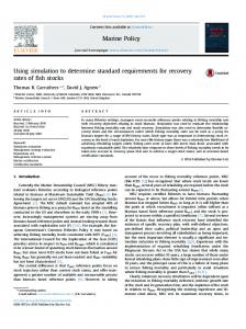
5. THE CASE FOR MULTIPLE RSS T VALUES IN A SINGLE IMAGE OR OVER A SHORT DURATION. Figure 2. Images 1-5 Side view of Bradley shows 5 images taken from 7:30pm to 9:48pm in November in Northern Michigan at Camp Grayling. The images are of an early version of the Bradley M2 and no longer reflect current

vehicle configurations. ViewIR, an infrared image analysis tool developed by Signature Research Inc, was used to calculate the vehicle mean and standard deviation, as well as the mean for several areas that could have represented the immediate background if the vehicle were positioned in different areas of the landscape. The bottom right image shows approximately the areas of interest that describes the vehicle and three different background areas (drawn in by hand and does not show the actual area, which did not include sky elements in the background for example). Chosen were the front of the vehicle, the side, and the trees behind the vehicle. Given the discussion above, one could ask why the foreground or even the side was used in this image, since it is probable that this ground was extremely disturbed during the testing process. This dataset was chosen for this paper not for its dramatic illustration of the point being made, but because of its potential for unlimited distribution. In addition, one could make the case that while this area would not be desirable for “the” one RSS T derived for the image if one were wishing to characterize the system in the traditional way, it is reasonable to say that such torn up terrain would be seen in battle and that it should be considered as one of the several RSS T cases that one might want to investigate as we develop this new process. There is also the fact that because of the close-in range imagery, we are limited to the amount of terrain surrounding the vehicle and have chosen where we can for the sake of the discussion.

Figure 2. Images 1-5 Side view of Bradley Figure 3 shows the results of the RSS T for each of the backgrounds for each image. The variability of RSS T within one image appears to be more dramatic in some images than others. Intuitively, we know that the higher the solar load on a terrain, the more variety there is in the scene, so it is not surprising that as the hour increases, the variability decreases. Figure 4 shows the data from the perspective of time. This figure reveals an interesting phenomenon to those who are not familiar with field testing: images taken within minutes of each other can show very different values (even worse than shown). Analysts not cognizant of this potential have assembled a stack of images, reduced them to RSS T values in the usual subjective manner, averaged them and delivered “the signature” of a system; all without describing the useful details and truthfulness of what was really going on with that system. Single Image RSS DT For a Given Vehicle- Left Side View 10.00

side of veh trees

RSS DT

8.00

foreground

6.00 4.00 2.00 0.00 1

2

3 Image

4

5

Figure 3. RSS T breakout by image

Bradley RSS DT Values Over 2 hours 9.00 8.50 8.00 7.50 7.00 6.50 6.00 5.50 5.00 4.50

foreground side of veh trees

7:2 7 7:5 8 8:2 8 8 9:0 9 9:3 9 6 P :40 P 5 P :09 P 4 P :38 P :52 P 7 P :21 P 6 P :50 P M M M M M M M M M M M

Figure 4. RSS T of side of vehicle broken out by time.

The example above was only for one side of the vehicle. To continue with the investigation, we repeated the analysis for the front of the vehicle as well, as shown in Figure 5.

Image 7 front view 7:43pm

Image 9. 8:37 pm

Image 8. 8:36pm

Image 10: 8:37pm < ?