ICOTS-7, 2006: Erickson
USING SIMULATION TO LEARN ABOUT INFERENCE Tim Erickson Epistemological Engineering, United States
[email protected] Many statistics educators use simulation to help students better understand inference. Simulations make the link between statistics and probability explicit through simulating the conditions of the null hypothesis, and then looking at sampling distributions of an appropriate measure. In this paper we review how we use simulation to help understand hypothesis testing, and lay out the relevant steps. We illustrate how using simulation and technology can make these difficult ideas more visible and understandable, through making processes more concrete, through unifying apparently disparate tests, and through letting the learners construct their own measures to study phenomena. INTRODUCTION Statistical inference is a tricky subject to learn. Inference is so hard that even professional researchers use it inappropriately. Why is inference so difficult to grasp? Partly because it’s a minefield of difficult, contrafactual ideas, not unlike the subjunctive mood in some languages. The idea of using simulations in teaching inference will be familiar to many readers. Why is it effective? It is easy to say simply, “because it makes things more concrete for the learner,” and that is true. But let’s look again, in order to draw our attention to some essential points. In this paper, we’ll focus on hypothesis testing. We start with a “polling” problem, which will lead us to a test of proportions. There is a proposition on the ballot in the upcoming election which, if passed, will make it legal to keep capybaras as pets. As president of the local Free the Capybaras League, you hope that this proposition will fail. In a poll of 50 likely voters, only 19 say they will vote yes. What does that tell you? Our first, naïve reaction is to be happy: only 38% of the voters are in favor of the proposition; surely it will fail. We decide to do a test of proportions, so we calculate z = –1.697, and find P = 0.09, so we are sad, remembering that we want P < 0.05. Then (after consulting with a statistician) we hear that we should have done a one-sided test, so that really P = 0.045, and we are happy again. We have used statistics blindly. In turning the crank on the test, we may not have understood what was going on, or the actual meaning of those P-values. One of the underlying concepts is that of the null hypothesis, which is hidden if you just calculate z and look up the results in a table. Another is the test statistic z itself: Why do we use it? Where does it come from, really? SIMULATING PROPORTIONS We can make things clearer if we make the analysis more concrete. We can do that through simulation. But what, precisely, should we simulate, and why? We have to ask what end result we really care about. In this case, we’re worried that even though the poll was 38%, the true proportion—and the end result—might be more than 50%. That figure 50% is the threshold, the situation that marks the border between success and failure. So we let 50% define our null hypothesis; we want to ask, if the true population proportion were 50%, how likely is it that we get a result as low as 38%? That is the contrafactual, subjunctive-mood question at the heart of this problem. And it is one we can answer empirically. If we use a (fair) coin to represent a voter, we can simulate a universe in which 50% of the voters are in favor of the Capybara Law. We say that “heads” means a person will vote “Yes” in the election. To simulate a poll, we flip the coin 50 times and record the results.
1
ICOTS-7, 2006: Erickson
Suppose we do that and get 23 heads. Does that mean our poll of 19 is so low that we can feel secure that the law will not pass? No. We have to do the simulation many times, and see where 19 falls in the distribution of poll results. The key point for students is that a single trial in this simulation is a poll of 50 voters, not an individual opinion. The relevant outcomes range from 0 heads to 50 heads, not from heads to tails. That is, the underlying intellectual structure of the situation is layered and hierarchical in addition to being contrafactual: students have to hold in their minds the individual voter and its representation (a single coin flip) as well as the model for a poll (50 coin flips and the result). So we flip 50 coins repeatedly, recording the numbers of heads, and plot the distribution of those results. Now we see that 19 is in the tail of the distribution, but not completely outside it. That is, it is possible, but unlikely, that if the population were evenly split (there’s that subjunctive again) we would get our result of 19. This is a key understanding students can get from simulation that too often eludes them when they approach the problem solely from calculation. In practical terms, however, if we flip 50 coins repeatedly, we will get tired before we build up a very large distribution. So we get computational help. Ignoring the exact mechanism for doing this—it is different for different programs—we use Fathom (Finzer, 2000) to simulate flipping 50 coins 1000 times. The resulting distribution appears in Figure 1. Histogram
Measures from poll 120 100 80 60 40 20
10
15
20
25 in_Favor
30
35
Figure 1: The results of 1000 polls of 50. Results with 19 or fewer “yes” votes are shaded somewhat darker; there are 52 such cases in this set of trials.
Our empirical result (this time) is P = 0.052. Let’s reflect on how this is the same and different from getting a traditional P-value. • Because of random variation, different students typically get different results for the same simulation. • There is no need to use a normal approximation; this simulation, by its nature, uses the binomial procedure. It doesn’t make much difference numerically, but conceptually, students do not have to worry whether the approximation is acceptable. • Students have to grapple with two N’s: the sample size (50) and the number of samples that contribute to the distribution (1000). The latter is not statistically relevant except that the empirical P-value will be closer to the theoretical as this N grows. • Perhaps most important, the simulation—or rather the process the students go through to get the results—makes it clearer what, precisely, the graph shows: the probability that you would get a result at least as extreme as the poll, if the population were evenly split. This also differs from the traditional test in that the student uses absolute numbers (19 out of 50) rather than proportions (p = 38%). Why would this matter? • The absolute number is more concrete, closer to the context. It is easier to imagine 19 people saying “yes” to capybaras than 38%. • With a clearer connection to the context, it’s easy to see that the relevant area is one tail rather than two. • Even though we want students to use proportional reasoning effectively, in this case the absolute numbers—both the numerator and denominator—are important conceptually. If
2
ICOTS-7, 2006: Erickson
1900 out of 5000 respondents said yes, it would still be 38%, but the meaning would be vastly different. (A Bayesian would point out that neither procedure gives us the answer we’re really interested in—the probability that the measure will fail—and that’s true. But we claim that at least in simulation, students are less likely to confuse (1 – P) with that value.) SIMULATING DIFFERENCE OF MEANS Let’s look at a different inference situation so that we can try to generalize. Suppose we want to test whether plants grow taller with plant food A than with plant food B. We measure each plant and store the value in a variable called height. Next, we construct a measure that tells how much taller the A plants are than B, for example, M = mean(height) from group A – mean(height) from group B. This value is our test statistic. The next—and critical—step is to scramble (or permute) the group memberships, leaving the height data alone, and compute the measure M on the scrambled data set. This simulates the null hypothesis: that group membership has no influence on height. We rescramble and compute this measure repeatedly, building up the sampling distribution to which we will compare our test statistic. This may be familiar to the reader as a “permutation test” or “randomization test,” and has an illustrious history going back to Fisher (1935) and Pitman (1937). Looking at both of these examples (the poll and the plants) we have an important insight: We have to simulate the situation in which the null hypothesis is true. Thinking about other examples we could just as well have described, a common structure emerges for hypothesis testing through simulation, which follows Gnanadesikan et al. (1987): 1. Collect data from the situation of interest—data that seem to reflect some phenomenon. 2. Design a measure of that phenomenon that you can calculate from the data. Ideally, this measure is a large number if the phenomenon is strong and present, and small—even zero—when the phenomenon is absent. The value for this measure, using the real data, is the test statistic. 3. Simulate the condition of the null hypothesis, and collect those data. 4. Compute the measure from simulated data, and repeat to build up a sampling distribution for the measure in question. 5. Compare the test statistic to the sampling distribution. The empirical P-value is the fraction of cases in the sampling distribution that are at least as extreme as the test statistic. These steps have special consequences for learning. Steps 2 and 3 are not mechanical; they both require some craft. To make such a simulation, a student has to design a measure, and has to figure out how to simulate the null. DESIGNING MEASURES If we are to build up a sampling distribution and compare a test statistic, we need a statistic. So the student must derive a single number from the experimental data that somehow expresses the phenomenon of interest. In the case of the plant food, the difference of mean heights makes sense. But we could also use the ratio of mean heights, or the difference in maximum heights, depending on what was most important. All that is required is a reliable way to calculate the statistic. Pedagogically, this is a constructivist’s dream. Students have to build a mathematical expression that embodies a meaning that they desire. They don’t need to use somebody else’s solution (Student’s t, for example), but later, when they are introduced to t (and chi-square and F), they will be able to see that these venerable and powerful statistics serve a purpose just as theirs do. This opens up the critical idea that we can compare how different statistics perform. Some are, after all, better than others at revealing the effects we are trying to study.
3
ICOTS-7, 2006: Erickson
It is also useful (and heartening) to see that if you do a test with a home-grown difference-of-means statistic, the P-values you get are about the same as you get if you use a t-test. Of course, t generalizes to any sample by assuming normality. This simulation procedure, on the other hand, assumes that the population distribution is the same as that of the sample, so a particular simulation works only for a particular data set. With computers, that lack of generality is not as important now as it once was. Furthermore, using simulation avoids abstractions that come with assuming normal distributions—abstractions such as degrees of freedom. Practically, it is often initially hard for students to get the idea that their statistic has to be a single number that describes what they are interested in, and that really it is a procedure for finding a number given any set of data. Perhaps this is because they are not looking ahead to the sampling distribution. SIMULATING THE NULL Even though each problem gives rise to its own specific model, there are common strategies for simulating a null hypothesis. As we have seen, polling suggests binomial trials with p = 0.5, whereas comparing two groups suggests scrambling. What about association? Interestingly, we can test for any sort of association using scrambling techniques. For example, if we have x and y values, and wonder if there is a correlation, it is really the same question as with the plants: is there a relationship between the two variables? We can use Pearson’s r (or any statistic we devise, parametric or no) as our test statistic. Then we scramble x or y and compute r for the scrambled data set. We do so repeatedly to build up the sampling distribution, and compare our test r to the distribution. The same logic applies to situations in which we would traditionally use a chi-square test or one-way ANOVA. Sometimes, a particular situation suggests a different simulation strategy. Fisher’s (1935) analysis of Darwin’s (1892) corn data is a good example. In that experiment, plants were paired in order to control for confounding variables. Each pair consisted of a self- and cross-fertilized plant of Zea mays. The conjecture was that the cross-fertilized plants would be generally taller. A relevant quantity is the difference of heights in each pair, so a suitable measure is the average or the sum of these differences. We could shuffle the heights of the plants, but here we are juggling three variables (fertilization, the “pair number,” and height) so we risk getting confused. Instead, Fisher used only the height difference within each pair, and, for the simulation step, randomly assigned an arithmetic sign to each value. A bit of reflection convinces us that this is equivalent to shuffling the fertilization “labels” within each pair, but from a student’s point of view, that equivalence may not be clear. Once we can accept the sign trick, the problems of getting the computer to do the simulation we want become much easier. It makes sense to use this randomization/sign strategy with many paired comparisons. THE ROLE OF TECHNOLOGY We have mentioned both computer simulation and manual simulation here; what is the role of each? Perhaps it is best to start with Freedman et al. (1997), who used a consistent metaphor of drawing slips of paper from a hat—a Gedankensimulation, if you will—to explain basic statistical concepts. This was especially effective because they could use the slip-drawing process as a unifying idea for many apparently dissimilar principles and techniques. When people first began using simulations in statistics education, computers were not as ubiquitous as they are today. We usually expected students to perform these simulations manually if at all. Students would roll dice, flip coins, or draw those slips of paper out of a hat. In some circumstances, they would look up numbers in a random-number table. Even in those far-away times, however, Gnanadesikan (1987) and his colleagues saw the promise of computers for speeding up the process, and the first bits of simulation software had already appeared. Extra speed is so alluring and fun, and makes so many things possible, that one is tempted to abandon manual simulations entirely. This is probably not a good idea, however: manual simulations—like using manipulatives and graphing by hand—give students hands-on experiences they can refer to as they move on to more abstract and technology-dependent activities. In addition to being more kinesthetic, manual simulations give students alternate representations for con-
4
ICOTS-7, 2006: Erickson
cepts, provide for collaboration with others, and, importantly, slow things way down, giving more time for thought. That said, usually simulation means simulation with technology. We expect that students will do enough manual simulation to understand the principles, and move on to the computer immediately after. Why? Because speed matters. There are three fundamental reasons this is so: • First, the speed of the computer makes it possible to do many more trials—and retrials— of a simulation than we could imagine doing by hand. • Second, the computer helps the student move up the ladder of abstraction. Without the speed, each of the 50 coin flips, or each of the shuffles, occupies our attention. With the speed, we can encapsulate the individual trials and focus on the sampling distribution. • Finally, the internal speed of calculation makes it possible for computers to display more about the process and results. This is more than just convenient or cosmetic. We see more and learn new things about the phenomena we’re studying, and about inference in general, when we use good technological tools. COMMENTS Others have written entire books about this (e.g., Simon 1993; Edgington 1995), so we will not press much further except to make a few comments. First, it is interesting to compare a student using a traditional approach with a student constructing a test using simulation. Traditionally, the student has to look at the variables, decide on a test, see if the data meet the requirements for the test, perform the relevant calculations or table look-ups, and interpret the results. In simulation, the number of things to be done is about the same. How do they differ? Simulation is more computing-intensive, and demands more creativity. And simulation may seem more unified: even though each measure may be different, and each null hypothesis must be simulated anew, the task simulate the null hypothesis is the same no matter what the form of the variables; a student may rightly get the impression that, at a deep level, a chi-square test is really the same as a two-sample t. After the equivalent traditional task, choose an appropriate test, the student can ignore the context completely, making the whole endeavor more abstract in a way that simulation does not. Second, we have been talking exclusively about hypothesis testing. The reader is probably familiar with bootstrapping as a technique for generating interval estimates that behave more or less like traditional confidence intervals. That is, we can use simulation (in this case, perhaps better called resampling) in many inference tasks—not just in hypothesis testing. Finally, the reference to bootstrapping highlights a commonality among many of the strategies we have mentioned so far. Whereas a traditional approach often assumes some distribution of the data—usually normal—and derives its results from the theoretical sampling distribution that arises under that assumption, a simulation strategy often implicitly assumes that the population has exactly the same distribution as the sample. As a consequence, worries about normality go away. (Worries about representativeness arise, of course, but are usually no worse than when using traditional tests.) CONCLUSION Why simulate? The first reason for us as teachers is that the entire process—simulating the null hypothesis, building up a distribution of statistics, and comparing our test statistic to that distribution—illuminates the underlying meaning of a hypothesis test. It replaces the struggle with the strange, subjunctive mantra (“…the probability that, if the null hypothesis were true, the statistic would be at least this extreme…”) with something more concrete: over here the null hypothesis is true. When students see that 52 times out of 1000, the statistic was as weird as they got in the actual experiment, they can reason more clearly about the meaning of their result. But, as we have seen, there are other advantages to using randomization tests as we have described them, especially: they don’t require normality; and they are effective with any reasonable statistic, even ones the students devise themselves. On the other hand, there is a great deal of inertia behind the tried-and-true parametric methods, which, after all, work well in many situations and are easy to use, even if they are often
5
ICOTS-7, 2006: Erickson
misinterpreted. And we, as teachers, have taught them before and know how. Simulation seems like a plausible educational tool, but there are challenges: designing measures; identifying and simulating the null hypothesis; understanding how to build up the sampling distribution; and interpreting the results. But as these factors change, and we learn to meet the challenges, the balance will shift for more and more teachers. It’s curious: Fisher (1935) used these methods (although looking at all possible permutations instead of a sample) to show that the time-saving parametric methods worked. Now computing has made simulation practical and fast. Stochastic methods are becoming more widely used professionally. So why do we need the traditional techniques? Will we eventually think of parametric methods as a brilliant but outmoded twentieth-century phenomenon? Will we think of them as tools we used to use, like log tables, the slide rule, and Napier’s bones? Probably not. We still teach calculus even though we solve most practical problems numerically. There is a beauty in crisp functional relationships—once we understand why they work—that contributes to our intuition about the phenomena we study. For example, the root-n that appears in so many formulas helps us think about the effects of sample size. As with so many things, then, we need to seek a balance. The concrete and practical leaven the abstract and analytical. The statistics course has long been too formal for most students. With technology, backed up by new thinking about how to use simulation effectively in education, we can create a new equilibrium, one that respects tradition but also opens doors for new understanding. ACKNOWLEDGEMENTS The author is grateful to Bill Finzer for useful comments and discussions, and to Key Curriculum Press for support in attending ICOTS. REFERENCES Darwin, C. (1892). The Effects of Cross and Self-Fertilisation in the Vegetable Kingdom. New York: D. Appleton and Co. [first published London, John Murray, 1876.] As digitized by Sue Asscher and John van Wyhe; the data appear at http://pages.britishlibrary.net/charles.darwin/texts/fertilisation/fertilisation06.html Edgington, E. S. (1995). Randomization Tests (3rd edition). NY: Marcel Dekker. Erickson, T. (2000). Data in Depth: Exploring Mathematics with Fathom. Emeryville, CA: Key Curriculum Press. Erickson, T. E. and Finzer, W. (1998). What to teach before inference: Building the bones from paper, software, and stories. In L. Pereria-Mendoza, L. S. Kea, T. W. Kee, and W-K. Wong (Eds.), Statistical Education - Expanding the Network: Proceedings of the Fifth International Conference on Teaching Statistics, Singapore. Voorburg: The Netherlands: International Statistical Institute. Finzer, W. (2005). Fathom Dynamic Data Software (Version 2). Emeryville, CA: Key Curriculum Press. Finzer, W. and Erickson, T. (1998). DataSpace -- A computer learning environment for data analysis and statistics based on dynamic dragging, visualization, simulation, and networked collaboration. In L. Pereria-Mendoza, L. S. Kea, T. W. Kee, and W-K. Wong (Eds.), Statistical Education - Expanding the Network: Proceedings of the Fifth International Conference on Teaching Statistics, Singapore. Voorburg: The Netherlands: International Statistical Institute. Fisher, R. A. (1935). Design of Experiments. New York: Hafner. Freedman, D., Pisani, R., and Purves, R. (1997). Statistics (3rd Edition). New York: W W Norton. Gnanadesikan, M., Scheaffer, R. L., and Swift, J. (1987). The Art and Techniques of Simulation. Palo Alto: Dale Seymour Publications. Pitman, E. J. G. (1937). Significance tests which may be applied to samples from any populations. Journal of the Royal Statistical Society, Supplement, 4, 119-130. Simon, J. L. (1993). Resampling: The New Statistics. Belmont, CA: Duxbury. (This book also comes with the software, Resampling Stats, http://www.resample.com.)
6