Using Sound to Classify Vehicle-Terrain Interactions in Outdoor Environments Jacqueline Libby and Anthony J. Stentz Robotics Institute Carnegie Mellon University Pittsburgh, PA 15213
[email protected],
[email protected]
Abstract— Robots that operate in complex physical environments can improve the accuracy of their perception systems by fusing data from complementary sensing modalities. Furthermore, robots capable of motion can physically interact with these environments, and then leverage the sensory information they receive from these interactions. This paper explores the use of sound data as a new type of sensing modality to classify vehicle-terrain interactions from mobile robots operating outdoors, which can complement more typical non-contact sensors that are used for terrain classification. Acoustic data from microphones was recorded on a mobile robot interacting with different types of terrains and objects in outdoor environments. This data was then labeled and used offline to train a supervised multiclass classifier that can distinguish between these interactions based on acoustic data alone. To the best of the author’s knowledge, this is the first time that acoustics has been used to classify a variety of interactions that a vehicle can have with its environment, so part of our contribution is to survey acoustic techniques from other domains and explore their efficacy for this application. The feature extraction methods we implement are derived from this survey, which then serve as inputs to our classifier. The multiclass classifier is then built from Support Vector Machines (SVMs). The results presented show an average of 92% accuracy across all classes, which suggest strong potential for acoustics to enhance perception systems on mobile robots.
I. INTRODUCTION Mobile robots that autonomously operate outdoors must be prepared to handle complex, unknown environments. At a minimum, these robots must be able to detect and avoid dangerous situations, which means their perception systems must be as accurate as possible. The fusion of data from different sensing modalities can increase accuracy, so it is important for roboticists to continue to explore the space of possible sensor choices. Typically, mobile robots use optical sensors to classify terrain in the surrounding environment. Microphones mounted on a mobile robot can complement optical sensors by enabling the vehicle to listen to the interactions that it has with that same terrain. Similar to other proprioceptive sensors, we propose to use acoustics as a means to help a robot understand what its body is experiencing. In this case, the experience is from vehicle-terrain interactions; hence, we will refer here to both acoustics and proprioception as “interactive” sensing modalities. Optical sensors such as cameras and lidar are powerful tools for classifying terrain in some volume of space around a robot. However, these systems are often unreliable due to variations in appearance within each terrain class. Interactive sensors will not be sensitive to changes in appearance. They might be unreliable due to other factors, but as long
(a) Vehicle in murky water
(b) Vehicle on gravel road
Fig. 1. The John Deere E-Gator platform used in this work is shown here at two data collection locations. (a) shows the vehicle in murky water. (b) shows the vehicle on a gravel road. These surfaces are somewhat similar in appearance, and many factors could change their appearance to the point where optical sensing will not be enough to distinguish between the two terrain types. On the other hand, the sound of the vehicle’s interaction with these terrain types would remain relatively constant.
as these are not the same factors that affect the optical sensors, then the two sensing modalities will fail in different circumstances. Therefore, they can be used to correct each other’s mistakes. Ideally, scene interpretation would always be achieved by the optical sensors so that the volume of space around the robot can be understood without the need for interaction with that volume. Interaction requires the robot to use resources such as energy and time; and for hazardous terrain types, interaction could damage the robot. However, if the optical sensors fail, then interaction might be the only alternative. Interactive sensors can at least alert the robot at the beginning of an unwanted event before further damage ensues or further resources are wasted. For instance, imagine that a robot has an optical classifier to detect water, but that this classifier sometimes makes mistakes. If the robot fails to detect the water and then subsequently drives into it, the sound of the water splashing could be used to correct the mistake. Allowing the robot to become wet could be damaging, but at least the splashing sound is a cue to slow down and retreat before the water gets deeper. Fig. 1 shows our robotic platform in two of our test environments. On the left, the robot is in a shallow stream; on the right, the robot is on a gravel road. These surfaces are somewhat similar in appearance, and many factors could change their appearance to the point where optical sensing will not be enough to distinguish between the two terrain types. These factors include variations in lighting conditions,
changes in consistency such as murky water, deformation of the water due to wind ripples or a running stream, and misleading facades such as surface vegetation or lily pads. They could confuse features coming from camera imagery such as color, intensity, and reflective properties. They could also confuse shape features coming from lidar, not to mention that lidar is particularly bad at handling water due to its reflective properties. On the other hand, none of these factors would have much of an effect on the sound of the vehicle’s interaction with these terrain types. There has been a body of work in terrain classification using proprioceptive sensors on mobile robots to interpret vehicle-terrain interactions. Wellington and Stentz [1] detected vegetation by using vehicle pose estimates to determine ground compressibility, and then used this to train a lidar model. Collins and Coyle [2] implemented vibrationbased terrain classification, using various inputs from an Inertial Measurement Unit (IMU) to distinguish between ground types such as sand, clay, grass, gravel and asphalt. In particular, they take care to characterize the body of the vehicle as a dynamic system, so that they can factor out the transfer function of the vehicle body. Brooks and Iagnemma [3] used a contact microphone to pick up vibrations coming from a wheel axle in order to distinguish between sand, grass and rock. Furthermore, they demonstrated selfsupervised terrain classification, using the vibration classifier to train a visual classifier. Note that the microphone they used is a contact microphone, which means it picks up vibrations through a solid, similar to the accelerometers in an IMU, rather than the normal air microphones we use in this work. Ojeda et. al. [4] did use an air microphone for terrain classification, but this modality is only able to distinguish grass. However, using an impressive suite of proprioceptive and near-range sensors, including microphones, gyroscopes, accelerometers, encoders, motor current, voltage sensors, ultrasonics and infrared, they are able to classify their full set of ground types: gravel, grass, sand, pavement, dirt. In this paper, we present a supervised multiclass classifier to distinguish between the different interactions a mobile robot can have with its environment. We extend the previous work in proprioceptive terrain classification with an in-depth analyzation of the use of microphones for this application. The results presented use only acoustic data. Similar to previous work, we analyze wheel-terrain interactions to identify certain ground types such as grass, pavement, and gravel. We extend the classification to body-terrain interactions pertaining to other parts of of the vehicle besides the wheels, which could indicate potential hazards. This includes the vehicle submerging into water and bumping up against large obstacles such as rocks. This paper is divided into the following sections. In Section II, we survey acoustic methods from other domains, since acoustic terrain classification on mobile robots is a relatively new application. In Section III, we lay out our technical approach, first describing the feature extraction methods derived from our survey and then describing our classification methods to build a multiclass classifier that can distinguish between a variety of vehicle-terrain interactions. In Section IV, we explain our experimental setup, where we describe the sensor setup on our test platform and
data collection in the field. In Section V, we present our results, which demonstrate an average of 92% accuracy across our classes, suggesting strong potential for acoustics to enhance perception systems on mobile robots. Conclusions and discussion of future work are presented in Section VI. II. RELATED WORK IN ACOUSTICS Acoustics used for listening to the interaction of one object with another has primarily been explored in controlled laboratory environments where single impacts are recorded. Wu and Siegel [5] placed microphones and accelerometers in the heads of hammers, which they tapped against sheet-like materials to determine their integrity. Durst and Krotkov [6] measured the sound of striking objects with canes and extracted spectral peaks as features to determine material type. In later work, Krotkov et. al. [7] and Amsellem and Soldea [8] performed similar experiments which also took the shape of the object into account and then determined material type based on spectral energy decay. This worked well for those applications in which the signal source was a single clean impact of a cane striking against a resonant object in a laboratory setting with no background noise. In our scenario, we sometimes have multiple impacts in succession (such as the vehicle bottoming out on rocks) or very complex impacts (such as splashing into water). In these cases, spectral peaks cannot easily be found. Furthermore, the vehicle is moving past these impacts as it is creating them, so the microphones will not stay in range of such impacts long enough to listen to their decay, even if the decay did have distinguishible features. There is also a body of work in contact-based acoustic sensing, where contact microphones are attached close to a source of impact to pick up vibrations through a solid. As mentioned previously, Brooks and Iagnemma [3] used a contact microphone placed on a wheel axle for terrain classification. Scanlon [9] used hydrophones on the human body to diagnose cardiac and respiratory functions for health status monitoring. Cohn et. al. [10] showed how a single acoustic sensor can be used on a home gas regulator to monitor gas usage and classify home appliances. Contact microphones are more similar to accelerometers than they are to air microphones because they sense impact through solid materials, either from transient forces or vibrations. With the use of air microphones, we can listen to a wider variety of interactions. For instance, the sound of tires splashing into water might not cause a vibration through the solid of the vehicle. Much of acoustic classification research in other domains has focused on finding structure within the time-varying elements of the data. Wellman et. al. [11] classified engine sounds by looking for harmonics in motor oscillations. This involves having a periodic sound source, which will manifest patterns over time. Hidden Markov Models (HMMs) have been used to learn the correlation of speech over time. (Nefian et. al. [12], Reyes-Gomez et. al. [13].) As mentioned previously, Krotkov et. al. [7] and Amsellem and Soldea [8] extract features from the spectral energy decay, where an evolution over time is one of the key factors. In our work we explicitly chose not to model time varying elements. There are no doubt dynamic changes in our data that could
form word-like structures, such as the start, middle and end of scraping against a rock, but we are not interested in learning the shape of one particular rock. Instead we want to generalize to any rock or other hard obstacle that could cause similar scraping sounds. It is generally true that the more complex a model is, the more of a chance there is for overfitting. This is especially true when data is limited. The only data we have for our application is data we collect ourselves; data collection and labelling is not easy, so we do not have very much of it. Our work is most similar to applications where: 1) air microphones are used, 2) continuous sounds rather than single-impact sounds are characterized, and 3) the continuous signal is treated as a stationary process. This is demonstrated by Hoiem and Sukthankar [14] and Giannakopoulos et. al. [15], where they looked at sounds from movies, such as dog barks, car horns, and violent content. Another example is from Martinson and Schultz [16], where a robot classifies voice signatures to help identify people. In all of these works, features were extracted by looking at short windows in time and characterizing the temporal and spectral characteristics of these windows. We take a similar approach in the work presented here. We split our recorded time signals into short windows, where each window is a data point in our set. We assume the signals to be stationary processes, treating each window as independent from other windows in the same sequence. Although there are dynamic elements to the signals we record, we purposely do not characterize them in order to generalize our classes, as discussed above. In the following section, we describe more specifically the features we use, which are inspired from the related work discussed above in these various other domains. III. T ECHNICAL A PPROACH In chronological order, our approach involves: 1) Collecting sound signals from different vehicle-terrain interactions 2) Hand-labeling sequences from each signal as belonging to a particular “class” or interaction 3) Splitting up each labeled sequence into short time windows 4) Extracting features from these windows 5) Training a classifier from these features 6) Predicting the labels of each window from the classifier 7) Comparing our predictions to the hand-labeled values A. Data Overview and Hand Labeling Data was collected for the vehicle interacting with terrains in different environments. Some of these interactions were benign, such as driving over a certain type of road; others represented hazardous situations, such as driving into water or hitting a rock. Section IV will discuss the data collection in more depth. To label the data, the starting and ending timestamps of each interaction event had to be determined. For example, a particular sound file might contain two events: driving through a puddle of water and driving along the road next to the puddle. Timestamps must be determined in order to break such a sound file up into separate sequences for these two events.
We developed interactive software to aid in labeling our data, which incorporates a combination of webcam images, time series plots, and audio feedback. A webcam was mounted on the vehicle near one of the microphones, providing a video stream of the environments that the vehicle was encountering (Fig. 2). Hand-labeling involved listening to the sound files and using time series plots of this data to visually zoom in on interesting sequences and graphically hand-select the starting and ending timestamps of each event. It is not always straightforward for a human listener to distinguish these events from just the sound information, so the webcam images were used as a second reference point. (The fact that our algorithms are successful only using sound data, while a human needs vision as well, speaks to the inherent power of sound as a computational tool.) Also, some terrain types were harder to label than others. For instance, driving through a puddle or hitting a rock are events that only last a short period of time, so we had to hand-label many of these events to have enough data for our algorithms. After labeling was complete, we had sequences of time series data where each sequence represented an event of interacting with a specific class. We split these sequences up into short time windows. Each window is then a data point which is used for feature extraction and classification. We empirically chose a window size of 400 ms, with 50% overlap between successive windows. We found that 400 ms was the shortest window we could use that still gave decent results. If the window is too short, then the small dynamic elements in the data will generate too much variability from one window to the next. As discussed previously, we are purposely not characterizing these dynamic elements. Another problem is that the shorter the window, the less frequency resolution that can be captured when transforming the window into the frequency domain. On the other hand, shorter windows allow detection to happen more quickly, which is important for the eventual goal of online algorithms for autonomous robots. B. Feature Extraction We thoroughly experimented with a wide array of feature extraction techniques. A few features are extracted from the time domain and the majority from the frequency domain. To obtain the frequency domain, we first smooth each time domain frame with a Hamming window, and then we apply a Fast Fourier Transform (FFT). We retain the spectral amplitude coefficients for further analysis, ignoring the phase. We normalize the signal first in the time domain and then in the frequency domain. In the time domain, we normalize the amplitude of the signal to range between [-1,1], and then in the frequency domain we normalize the spectral distribution to sum to 1. Normalization makes our algorithms blind to volume, which prevents the classifiers from overfitting to factors such as the capture level of the microphone, the specific microphone being used, the distance from the microphone to the sound source, and certain variations across events from the same class. We extract three features from the time domain. The first is the zero crossing rate (ZCR), which is the number of times per second that the signal crosses the zero axis. The second is the short time energy (STE), which is the sum of the
squares of the amplitudes. The third is the energy entropy, which is a measure of the abrupt changes in energy present in the signal. To calculate the entropy, the frame is subdivided into k subframes, with k = 10, chosen experimentally. The energy of each subframe is calculated as the short time energy (described above), and then normalized by the energy of the whole frame. The entropy is then calculated PK−1 by E = − i=0 σ 2 · log2 (σ 2 ) where σ is the normalized energy of a subframe. We extract many features from the frequency domain. The most direct is treating each coefficient in the raw spectrum as a dimension in a feature vector. Because our microphone has a sampling frequency of 44.1 kHz, using the entire spectrum is computationally overwhelming. The majority of the spectral power is under 2 kHz, so we experiment with only using the lower part of the spectrum, varying the truncation point between 0.5 and 2 kHz. The rationale for this comes from the fact that the signal-to-noise ratio (SNR) is lower in regions of the spectrum where there is less power. However, these low SNR regions could contain some information, and this information might be very pertitent to distinguishing between different classes, so we do not necessarily want to ignore these regions altogether. Therefore as an alternative feature vector, we bin the spectrum along the coefficients, as is discussed in Hoiem and Sukthankar [14] and Peeters [17]. Binning allows the entire spectrum to be captured while still reducing the dimensionality. We also experiment with bins that are spread log-uniformly along the frequency scale, which focuses on the lower frequencies. This technique is particularly useful in capturing the entire spectrum and focusing on the high SNR regions, while still reducing the dimensionality. We experiment with different bin sizes for linear scaling and different logarithmic bases for log-uniform scaling. Instead of looking at the entire spectrum as a vector, we also experiment with scalar features that characterize the shape of the distribution. We compute the moments of the distribution: the centroid, standard deviation, skewness, and kurtosis. (See Wellman et. al. [11] for equations.) We also compute the spectral rolloff, which is the frequency value under which a certain percentage of the total power lies. We use a value of 80%, determined empirically. We also compute the spectral flux, which measures the rate of energy change. The flux is computed by taking the difference between the coefficients of consecutive frames and then summing and squaring the differences. The various scalar quantities presented above are combined into feature vectors. Giannakopoulos et. al. [15] looks at six of these scalars in particular: ZCR, STE, energy entropy, spectral centroid, spectral rolloff, and spectral flux. In following these methods, we combine these scalar values into a 6D feature vector. Wellman et. al. [11] looks specifically at the distribution moments of the spectrum, and in following these methods, we create a 4D feature vector consisting of the spectral centroid, standard deviation, skewness and kurtosis. To summarize, we take each 400 ms frame as a data point, and process it in different ways to form various feature vectors. We delineate these vectors in the following list, which are each used in separate trials as inputs into our
classification algorithms. • Raw spectral coefficients, truncated at varying values. • Bins of spectral coefficients, with varying methods for binning. • 6D vector of temporal and spectral characteristics, derived from Giannakopoulos et. al. [15], which we will refer to as the “gianna” features. • 4D vector of spectral moments (“shape” features). • 9D vector which combines the 6D and 4D vectors above. We call this the “gianna and shape” vector. (Note that this is not 10D because one of the dimensions is present in both original vectors.) C. Classification For classification, we use Support Vector Machines that are implemented in the SVM-Light library (Joachims [18]). Since this is a new form of mobile robot proprioception, we do not have previous datasets to work from. The datasets we collected are small in comparison to the online data banks from which many machine learning applications benefit. SVMs are a good choice for handling small datasets because they are less prone to overfitting than other methods. SVMs also have a sparse solution, allowing for predictions to be very fast once the classifier is trained. This is important for online applications such as mobile robotics. (See Burges [19] for more discussion on these motivations.) We experiment with both linear and radial basis function (RBF) kernels. RBF kernels sometimes perform better than linear kernels because they can handle non-linear separations, and they sometimes perform better than polynomial kernels because they have less parameters to tune and less numerical instability. Linear kernels, however, are sometimes better for high dimensional feature spaces. We build a multiclass classifier with the standard onevs-one approach: we train binary SVMs between each pair of classes, and then each binary classifier is a node in a Decision Directed Acyclic Graph (DDAG), as described in Platt et. al. [20]. A nice analogy for the DDAG graph is the following: imagine you have a game with multiple players. In each round of the game, two of the players compete. (This competition between two players represents a binary node.) Whichever player loses the round gets kicked out of the game. The winner then competes against another player, and the process repeats until there is only one player left in the game. The best way to use SVMs for multiclass classification is an open question. We choose the one-vs-one approach (as opposed to using a single multiclass SVM) so that we can decompose the problem into a series of simpler problems. It is also faster in training time than a single multiclass SVM, which allows us to experiment with many different hyperparameters and feature combinations. One-vsrest is another decomposition technique, but this approach involves another layer of parameter fitting to resolve the differing scales between binary nodes. With that being said, decomposition methods such as one-vs-one and one-vs-rest are both popular techniques, and standard SVM libraries such as LIBSVM and Weka use these techniques respectively for their multiclass implementations. As a benchmark comparison, we also use k-nearest neighbor (k-NN) with inverse distance weighting. We use k = 10,
which was determined empirically. This means that for each binary decision in the DDAG tree, we replace the learned SVM classifier with a k-NN classifier. IV. DATA COLLECTION Data was collected from microphones mounted on a vehicle that was manually driven through various outdoor environments. The vehicle used was a mobile robot built on a John Deere E-Gator platform shown in Fig. 1. Two microphones were used, one mounted on the front grill of the vehicle (Fig. 2), and one mounted on the back bed (Fig. 4). A webcam is also mounted on the front of the vehicle to provide image streams to assist in hand-labeling. Data was collected for six outdoor vehicle-terrain iteractions, each of which is categorized as a separate class in our classification algorithms. The classes fall into two main categories: benign and hazardous terrain interactions. We have three classes for each category, as listed below: 1) Benign terrain interactions: a) Driving over grass b) Driving over pavement c) Driving over gravel road 2) Hazardous terrain interactions: a) Splashing in water b) Hitting hard objects c) Wheels losing traction in slippery terrain The benign interactions are different types of flat surfaces that the vehicle might drive over, whereas the hazardous interactions represent dangerous situations that a vehicle might encounter with caution or by accident. For each class, we collected data from multiple locations. We chose locations with differing characteristics so that there was variation within each class. This prevented our classifiers from overfitting to specific data sets. For the benign terrains, the sounds differed according to how the tires interacted with the road surface. For the grass terrain, the locations varied from clean-cut lawns to unmaintained, park-like settings. For the pavement terrain, the locations varied from new asphalt parking lots to older concrete roads. For the gravel terrain, the locations varied from dirt roads with a few slag pebbles to dense collections of crushed limestone.
Fig. 2. The front grill of the E-Gator platform, showing where sensors are mounted. Close-ups are shown for one of the microphones and the webcam attached to the front grill. The microphone is positioned to monitor interactions between the front of the vehicle’s body and the environment. The webcam collects an image stream which assists in hand-labeling.
(a) Puddle of water
(b) Stream with running water
Fig. 3. Examples of various environments used for the “splashing in water” class, speaking to the ability of the classifiers we train to generalize across varying environments within each class.
For the “splashing in water” terrain, we drove into puddles and shallow streams to collect the sound of splashing produced by the tires and undercarriage of the vehicle. We collected data from three puddles formed from rain in ditches along dirt roads (Fig. 3(a)), where the dirt roads had varying levels of mud and ditch depth. We also collected data from two locations in a naturally running stream of water about one foot deep (Fig. 3), where each location had varying levels of terrain roughness and water flow. For the “hitting hard objects” terrain, we drove the side of the vehicle into large rocks and other hard objects (Fig. 4). To prevent damage to the vehicle, we rigidly attached a large steel sheet to the side of the vehicle, similar in thickness and material to the vehicle frame. The collisions always happened against this steel sheet. We collected data from six different objects, hitting each object multiple times from multiple angles. Our data set contains 20 to 30 collisions with each object, consisting of banging and scraping sounds as the vehicle hits the object and continues to try to drive past it. We used objects of various shapes and sizes. One was a rectangular cement block, two were sandstone rocks, two were rocks formed from a concrete gravel mix, and one was a rock formed from molten slag. For the “losing traction” class, we collected data when the vehicle got stuck in slippery terrain such as mud or snow, or from uneven terrain such as a ditch. These events consisted of the tires spinning in place with no traction. This data was the result of our vehicle actually getting stuck when trying to
Fig. 4. Example of a rock used for the “hitting hard objects” class. Left: The vehicle driving into a rock. The location of the collision is against the steel metal plate mounted to the side of the vehicle, to protect the vehicle’s frame from damage. Right: A closeup of the microphone mounted on the back of the vehicle near to the collision location.
collect data for other classes. We captured this data type in over ten different locations, with each location consisting of multiple traction loss events. These locations included ditches in off-road meadows, ditches in a snow-covered trail, uneven terrain in the stream mentioned above, and various ditches next to the rocks mentioned above. The two microphones used were identical, differing only in color. They are Blue Snowball condenser microphones, with a 44.1 kHz sampling rate and a 16 bit depth. We used the omnidirectional setting on both microphones so that our data generalized to sounds captured from different locations on the vehicle. The back microphone was positioned near the mounted steel sheet so that we could capture the sounds of hitting hard objects. The front microphone is mounted low to the ground near the front wheels. This microphone was predominantly responsible for capturing the sounds for all of the other classes. For all of the trials, we maintained a roughly constant speed between 2 m/s and 3 m/s. Earlier experiments showed that speed can have a large effect on the sound of the interaction, so we control this variable here. We implemented a speedometer by differentiating the encoder values and displaying them to a laptop screen, which the driver uses to roughly control the speed. V. EXPERIMENTS AND RESULTS We separated the data for each class into training and test sets. Since we have multiple locations for each class, we never have the same location in both the training and test sets for any given class. Our results therefore prove the ability of our models to handle new locations. Table I shows the number of data points in each of the sets. Note that there is much less data for the last two classes because these interactions involved short events, whereas for the first four classes we had more continuous stretches of terrain with which to interact. To preserve symmetry, we trained on the same number of data points for each class. Since 89 was the minimum number of training points, we randomly chose 89 points from the larger data sets to use for the training. We did not limit the test data. We ran our algorithm on separate trials for different feature and classifier combinations. We experimented with the five feature sets as listed in Section III and three classifier variants: SVM with an RBF kernel, SVM with a linear kernel and k-NN. For each combination, we trained the binary classifiers separately, where each binary classifier is a node in the one-v-one graph. (This does not apply to the k-NN classifier, since there is no training involved.) For each binary node, we performed the following steps. First, we zero mean shifted and whitened the training data.
These transformations were stored as part of the model for that node and then used as well on the test data. We then used leave-one-out cross validation on the training data to tune the constraint parameter for the SVM as well as the sigma value when using an RBF kernel. We iterated over values between 2e-5 and 2e11 for each parameter, first over a course grid and then again over a finer grid using the optimal subregion from the course grid. Once the training on the binary nodes is complete, the test data is fed into the one-v-one graph, and accuracies are determined by comparing the true labels to the predictions that are output from the graph. Fig. 5 shows accuracies for each of the feature/classifier combinations. Full results would show a 6x6 confusion matrix for each trial. For compactness, we condense each confusion matrix into one number, which is the average of the true positive rates across all six classes. Note that for a binary classifier, 50% accuracy signifies no information. Across six classes, this number is 17%. The lower the performance of a trial, the more that classifier is overfitting to the training data. The worst results are given by the raw FFT feature vector. Since this vector has the highest dimension, it makes sense that it would overfit. The “log bins” vector overfits with the RBF kernel but then performs very well with the linear kernel. This is plausible considering this vector still has a relatively high dimension; since the RBF kernel adds another parameter to the classifier, this increases the chances of overfitting. The lower dimensional feature sets perform well across both SVM variants. The two trials that perform the best are the “gianna and shape” feature set with an RBF kernel, and the “log bins” feature set with a linear kernel. We use these two combinations to run further experiments. The next factor we experimented with was which microphone to use. The easiest method is to always use the back microphone for the “hitting hard objects” class, and use the front microphone for all other classes. This means that for both the training and test sets, we explicitly select which microphone to use. This is what we did for the results presented above in Fig. 5. One could argue that this is giving the test data too much information, so we also ran experiments where we use both microphones for all classes. This means that for each short time window in our data set, we really have two short time
TABLE I N UMBER OF DATA P OINTS FOR EACH C LASS class grass pavement gravel water hard objects losing traction
training 1364 1856 3986 1787 203 89
test 1373 1377 4347 3384 65 244
Fig. 5. Bar chart of average accuracies for the different feature and classifier combinations. Each main group along the x-axis is a classifier choice. Within each group, the legend specifies the various feature sets used. The dimension of each feature choice is given in parentheses.
windows, one from each microphone. We experiment with different methods of combining these two data points. One way is to treat the two data points as separate members of the dataset, which doubles the number of data points. Another way is to concatenate the feature vectors from the two data points together, thereby doubling the dimension. A third way is to average the two vectors together. We try each of these methods on the two best trials from above, and we show these results in Fig. 6. Again, each bar is an average true positive rate for a particular trial. The first group on the left, “choosing mic”, is the original method of choosing which microphone to use for which class, and so these two bars are the same as in Fig. 6. The next three groups show the different methods of combining the two microphones. The averaging method performs the best. Doubling the dimension also performs very well for the “gianna and shape” vector, but the “log bins” vector suffers. Since the “log bins” vector already has a very high dimension, it makes sense that doubling the dimension would cause problems. Treating the microphones as separate data points (“doubling data”) does not perform very well because the data coming from each microphone is inherently different. The distance from a particular sound source should not in itself have much of an effect since we normalize the volume, but the ratio of source sound to background sound will be quite different for the two microphones. We take the best result from above that uses both microphones (“averaging” with “gianna and shape”), and we further improve the results by applying a mode filter to smooth out noise. Each short time window exists within a time sequence, and we slide a larger window across each sequence that is five times the size of each short time window data point. We tally the votes for each data point’s prediction in this larger window, and use this vote to relabel the data point in the center of the window. Note that even though we are using the time dimension to help with noise smoothing, we are still ignoring this dimension in the training process so that the time-varying structure is not modeled.
This smoothing step increases the average accuracy from 78% to 92%. We show the full confusion matrix for this best result after smoothing in Table II below. The class that performs the worst is the pavement class, with a true positive rate of 70%. This class is getting confused the most with the other benign road classes, the grass and the gravel. This suggests that the differences in the sounds between these road classes are more subtle. If the motivation is to detect hazardous situations for the vehicle, then we might collapse the benign road types into one general benign class. Without retraining, we can convert the matrix to combine the benign classes into one block cell. This gives us the 4x4 matrix in Table III below. Collapsing these three classes is equivalent to the classifier adding an “or” operation after its prediction step. In other words, the “benign” class is chosen if the grass class or the pavement class or the gravel class is predicted. This increases the average accuracy to 96%, with a minimum class accuracy of 92%. We summarize here how we arrive at our final results. We use a “gianna and shape” feature vector, averaging the feature vectors coming from each microphone. We feed the averaged vector as a data point into an SVM classifier with an RBF kernel. This classifier is trained separately for each binary node in the multiclass graph. We then smooth out noise by running a mode filter over the predictions. This gives us an average accuracy of 92%, and we can optionally perform a final “or” operation to collapse the benign road classes, giving us an average accuracy of 96%. VI. CONCLUSIONS AND FUTURE WORK In this paper, we present a method to classify the different interactions a mobile robot can have with an outdoor environment, using only acoustic data. We present acoustics as a new type of proprioceptive technique for mobile robots to “feel out” their environment. To the best of the author’s knowledge, acoustics has not been used before for classifying a variety of environmental interactions, so we draw from research in other domains to formulate our methods. We survey past research in mobile robot proprioception as well
Predicted
TABLE II C ONFUSION M ATRIX FROM THE T RIAL WITH THE B EST AVERAGE ACCURACY OF 92% paved 9 70 19 1 0 1
Actual Label gravel splash 1 1 1 0 97 2 0 96 0 1 1 0
hit 0 0 2 0 98 0
slip 0 0 1 2 5 92
TABLE III C ONFUSION M ATRIX WITH BENIGN CLASSES COLLAPSED , INCREASING AVERAGE ACCURACY TO 96%
Predicted
Fig. 6. Bar chart of the average accuracies for different ways of combining data from the two microphones. The two best features/classifier combinations are depicted in orange and red. Each main group along the x-axis specifies a different way of combining the data. The left-most group, “Choosing mic” means that the microphone was hand-chosen for each class. The next three groups are different ways of blindly taking data from both microphones. “Doubling data” means that the windows from each microphone are treated as separate data points. “Doubling dimension” means that the feature vectors from each microphone are concatenated together into a vector double the size. “Averaging” means that the two feature vectors are averaged together.
grass paved gravel splash hit slip
grass 98 0 1 0 0 1
benign splash hit slip
benign 99 0 0 1
Actual Label splash hit 3 2 96 0 1 98 0 0
slip 1 2 5 92
as acoustics used in other applications. We weigh the similarities and differences of these other applications in order to choose the right techniques for our domain. We obtained an average true positive rate of 92%, and this rate was increased to 96% when focusing on hazardous terrain interactions. (Future work could include improving the accuracy for the benign terrain types.) These are very strong results and suggest that acoustics is a promising method for enhancing the perception systems on mobile robots. Currently our method works on 400 ms windows, with smoothing across five windows, so detection is automatic to within a range of 2 seconds. For detecting hazardous classes such as water, 2 seconds might be too long of period to wait, so these techniques could be improved by decreasing the detection time. Although we achieve good accuracy for six labels, future work could continue to expand this label set to include more terrain types. Along with an expanded label set comes the need to continue to explore feature extraction and classification techniques. Although SVMs are a good choice for small data sets, other classifiers might lend themselves more naturally to large multiclass problems. This work is our first attempt at feature selection, first qualitatively by surveying other acoustic research and selecting suitable choices, then quantitatively by analyzing different feature choices and classifier variants. These choices can be used as a benchmark to build more complete feature selection techniques, using formal methods to maintain computational feasibility in the selection process. From a hardware perspective, this work would benefit from incorporating other proprioceptive sensors for classification, such as vibration sensors, IMUs, gyroscopes, GPS, and various near-range sensors. One simple proprioceptive parameter is speed, which we mentioned has a large effect on the acoustic signature of the vehicle-terrain interactions. We controlled this parameter by manually driving the vehicle at the same speed for all of our experiments. Future work could involve autonomous speed control and then data collection at more specific discrete speed increments. This data could then be used to either train separate classifiers for each speed or more intelligently interpolate between speeds to factor out this variable. Other parameters besides speed should also be examined, and then incorporated either as a control or as an input to the terrain classifier. As the number of sensing modalities increases, so too does the number of data fusion techniques. Not only is feature selection important, but feature combination becomes important as well. Future work could explore how to combine different feature vectors, whether they are vectors coming from different data sources or vectors coming from different feature extraction methods on the same data. The areas of enhanced perception and sensor fusion are rich with research questions and are particularly useful for robotic applications that involve large amounts of uncertainty, such as mobile robots driving in outdoor environments. VII. ACKNOWLEDGMENTS This work was conducted through collaborative participation in the Robotics Consortium sponsored by the U.S Army Research Laboratory under the Collaborative Technology
Alliance Program, Cooperative Agreement W911NF-10-20016. The views and conclusions contained in this document are those of the authors and should not be interpreted as representing the official policies, either expressed or implied, of the U.S. Government. The authors would also like to thank Hatem Alismail and Debadeepta Dey for software collaboration at the start of this project, as well as Scott Perry for help with field experiments, Don Salvadori for mechanical fabrication, and Sean Hyde for computer engineering support. R EFERENCES [1] C. Wellington and A. Stentz, “Online Adaptive Rough-Terrain Navigation in Vegetation,” in IEEE International Conference on Robotics and Automation (ICRA), 2004. [2] E. J. Coyle and E. G. Collins, “A Comparison of Classifier Performance for Vibration-based Terrain Classification,” in 26th Army Science Conference, 2008. [3] C. A. Brooks and K. Iagnemma, “Self-Supervised Terrain Classification for Planetary Surface Exploration Rovers,” Journal of Field Robotics, vol. 29, no. 1, 2012. [4] L. Ojeda, J. Borenstein, G. Witus, and R. Karlsen, “Terrain Characterization and Classification with a Mobile Robot,” Journal of Field Robotics, vol. 23, no. 2, 2006. [5] H. Wu and M. Siegel, “Correlation of Accelerometer and Microphone Data in the Coin Tap Test,” IEEE Transactions on Instrumentation and Measurement, vol. 49, no. 3, 2000. [6] R. S. Durst and E. P. Krotkov, “Object Classification from Analysis of Impact Acoustics,” in Proceedings of the IEEE/RSJ International Conference on Intelligent Robots and Systems (IROS), 1995. [7] E. Krotkov, R. Klatzky, and N. Zumel, “Robotic Perception of Material: Experiments with Shape-Invariant Acoustic Measures of Material Type,” in International Symposium on Experimental Robotics (ISER), 1996. [8] A. Amsellem and O. Soldea, “Function-Based Classification from 3D Data and Audio,” in Proceedings of the IEEE/RSJ International Conference on Intelligent Robots and Systems (IROS), 2006. [9] M. V. Scanlon, “Acoustic Sensor For Health Status Monitoring,” in IRIS Acoustic and Seismic Sensing, 1998. [10] G. Cohn, S. Gupta, J. Froehlich, E. Larson, and S. N. Patel, “GasSense: Appliance-Level, Single-Point Sensing of Gas Activity in the Home,” in IEEE International Conference on Pervasive Computing and Communications (PerCom), 2010. [11] M. C. Wellman, N. Srour, and D. B. Hillis, “Feature Extraction and Fusion of Acoustic and Seismic Sensors for Target Identification,” in SPIE Peace and Wartime Applications and Technical Issues for Unattended Ground Sensors, 1997. [12] A. V. Nefian, L. Liang, X. Pi, L. Xiaoxiang, C. Mao, and K. Murphy, “A Coupled HMM for Audio-Visual Speech Recognition,” in IEEE International Conference on Acoustics, Speech, and Signal Processing (ICASSP), 2002. [13] M. Reyes-Gomez, N. Jojic, and D. P. W. Ellis, “Deformable Spectrograms,” in AI and Statistics, 2005. [14] D. Hoiem and R. Sukthankar, “SOLAR: Sound Object Localization and Retrieval in Complex Audio Environments,” in IEEE International Conference on Acoustics, Speech, and Signal Processing (ICASSP), 2005. [15] T. Giannakopoulos, K. Dimitrios, A. Andreas, and T. Sergios, “Violence Content Classification Using Audio Features,” in Hellenic Artificial Intelligence Conference, 2006. [16] E. Martinson and A. Schultz, “Auditory Evidence Grids,” in IEEE/RSJ International Conference on Intelligent Robots and Systems (IROS), 2006. [17] G. Peeters, “A Large Set of Audio Features for Sound Description (Similarity and Classification) in the CUIDADO Project,” 2004. [18] T. Joachims, “Making Large-Scale SVM Learning Practical,” in Advances in Kernel Methods - Support Vector Learning, B. Sch¨olkopf, C. Burges, and A. Smola, Eds. MIT Press, 1999. [19] C. J. C. Burges, “A Tutorial on Support Vector Machines for Pattern Recognition,” Data Mining and Knowledge Discovery, vol. 2, no. 2, 1998. [20] J. C. Platt, N. Cristianini, and J. Shawe-taylor, “Large Margin DAGs for Multiclass Classification,” in Advances in Neural Information Processing Systems (NIPS), 2000.