Natural Terrain Classification using 3-D Ladar Data - Robotics Institute
Recommend Documents
tedious labeling process is performed using 3D Studio Max which allows to select 3-D .... separation between laser sweeps is 2. 3 of a degree over 115 .... [11] J. Albus and al., â4d/rcs sensory processing and world modeling on the demo iii ...
Jun 7, 2006 - Figure 1: Real-time data processing for scene interpretation. .... a related field, a large literature exists on the recovery of the ground terrain surface from airborne laser ...... Our code runs on a Linux computer, either a VME.
Aug 6, 2006 - harder it is to discern rules that broadly apply. Nonlinear relationships .... that fall between two planes emanating from the vehicle's control point ...
Carnegie Mellon University ..... We empirically chose a window size of 400 ms, with 50% ... which is important for the eventual goal of online algorithms.
The parts from all models are then grouped ... objects in a class (e.g., all pickups have a truck bed). Clas ..... IEEE Trans. on Systems, Man, and Cybernetics, Part.
Data-driving Algorithms for 3D Reconstruction from Ladar Data. Gerard Berginc1, Ion Berechet2, and Stefan Berechet2. 1Thales Optronique S.A., 2 Avenue Gay ...
aligning multiple 3D data sets in a common coordinate system. In existing ..... The large number of FSV pixels indicate an incorrect match. Fig. 7. The distribution ...
application, which we call hand-held modeling, the object to .... the object before a laser scanner (left), we obtain 3D data from various viewpoints (center),.
(XUV) (shown in Figure 1) can autonomously navi- ... Optics LAser Detection And Ranging (LADAR), color .... for the adaptive thresholding of the distance Dmax is given below: if µ < D ... Calculate H= ... The LADAR was mounted on a pan/tilt.
Abstract - This paper presents a laser-based hazard detection system for rovers ... depressions, the laser system contributes to the overall safety by sensing ...
Usually, the terrain classification procedures are based only in the heights of the area contained ... classification using the information derived from the statistical.
Our CGP for Image Processing (CGP-IP) system quickly .... OpenCV image processing library functionality [5]. With .... able C# or C++ code based on OpenCV.
Oct 15, 2006 - vectors and a combination of this representation with the PSD. We train and classify the ..... The best performance was achieved by the feature ...
label probabilities from the tile-level aspect models, an efficient. 17 .... (a). (b). Fig. 2. Two training tiles with (a) keyword-level labeling and (b) corre- sponding ...
Wolfram Burgard. Department of Computer .... projected into 3D Cartesian space using standard geometry. ... output is range measurement, which has to be converted into ... One can use HMM also to learn the parameter of the model λ, but in ...
sensor data and uses feedback from terrain contact to increase accuracy. .... bal maps, the current body frame for leg recovery, and future ... sion or bad data in the range image. .... that occurred during the experiment was an intermittent hard-.
Dec 7, 2016 - The Unity 3D game engine was used as the main platform for developing the system due to its ..... http://www.apptelemetry.com/index_en.html.
Dieter Fox. University ... labeled training data by leveraging data sets available on the. World Wide .... beling individual laser points, our system labels a soup of.
application of such a system, the ideas can easily be ... infrared is a cheap means of accumulating data with high .... A software developers kit allows us to ...
We have developed a multiplatform telesupervision architecture that supports .... For the mobile deployment of freshwater quality sensors, a fleet of small and ...
Keywords SARTM .Terrain. P. P. Patel ( ) . A. Sarkar. Department of Geography, Presidency College,. Kolkata -700073, India e-mail: [email protected].
semantic segmentation [23, 7, 21], object detection [4, 13, 9] and moving object ... Fully Convolutional Network based method [13] for detect- ing objects, where ...
[2] N. Schliep-Andraschko F.M. Andraschko, A. Krekeler. Terminologie, Klassifikation und computergestuetzte Bearbeitung der. Keramik des 1. Jahrtausends v.
Natural Terrain Classification using 3-D Ladar Data - Robotics Institute
of ladar data using local 3-D point statistics into three classes: clutter to capture ... on the recovery of the ground terrain surface from airborne laser sensor, see [5] for .... a linux laptop and we communication with the robot using. NML buffers via ...
Natural Terrain Classification using 3-D Ladar Data Nicolas Vandapel, Daniel F. Huber, Anuj Kapuria and Martial Hebert Carnegie Mellon University 5000 Forbes Avenue Pittsburgh, PA, USA Email: [email protected]
Abstract— Because of the difficulty of interpreting laser data in a meaningful way, safe navigation in vegetated terrain is still a daunting challenge. In this paper, we focus on the segmentation of ladar data using local 3-D point statistics into three classes: clutter to capture grass and tree canopy, linear to capture thin objects like wires or tree branches, and finally surface to capture solid objects like ground terrain surface, rocks or tree trunks. We present the details of the method proposed, the modifications we made to implement it on-board an autonomous ground vehicle. Finally, we present results from field tests using this rover and results produced from different stationary laser sensors.
I. I NTRODUCTION Autonomous robot navigation in vegetated terrain remains a considerable challenge because of the difficulty in capturing and representing the variability of the environment. Although it is not a trivial task, it is possible to build models of smooth 3-D terrains like bare ground. But it is much more difficult to cope with areas that cannot be described by piecewise smooth surface like grass, bushes, or the tree canopy. Because they exhibit porous surfaces and random medium of propagation in their interior they are more naturally described by 3-D texture rather than by smooth surfaces. In this paper, we present a method to segment 3-D point clouds, acquired by a laser radar, into three classes: surface (ground bare terrain surface, solid object, large tree trunk), linear structures (wires, thin branches) and scatter (tree canopy, grass). Similar points are then grouped into consensus region corresponding to large pieces of surfaces. Our method does not rely on a specific sensor geometry or scanning pattern. In particular the internal representation is updated every time a new data point is acquired by the sensor, irrespective of the order of acquisition. We use statistical classification techniques, and we learn most of our method parameters using training data sets manually label, reducing the amount of hand tuning. We presented in [1] results produced off-line using data coming from different laser radar sensors in a variety of environments. In this paper we present results from onboard processing on the General Dynamics Robotic Systems eXperimental Unmanned Vehicle (GDRS XUV) as well as additional results from stationary laser radars. Because of its importance for obstacle detection and environment modeling, the issue of detecting and segmenting vegetation has been explored in the past. The use of spectral data has received a lot of attention compared to the use of geometric information. A few approaches, pioneered by Mumford [2], considered single point statistics of range image
of natural environments. But to characterize texture we need local statistics on range, derivative of ranges and frequency components. In robotics, Matthies [3] presented results on single point statistics computed from data from a single point laser range finder, to differentiate between vegetation and solid surface like rocks. In [4], he presented a more geometric approach to this problem. A large literature exists on the recovery of the ground terrain surface from airborne laser sensor, see [5] for a review and comparison of the methods. This includes the filtering of the vegetation and the interpolation of the terrain surface. In robotics, Lacaze [6] measured the permeability of the scene to detect vegetation. A similar approach is used by Wellington in [7], in addition to other methods, to recover the load bearing surface. Below we present our approach to the problem of 3-D data segmentation, the implementation we produce to run on-board the XUV and finally results from different stationary sensors and results from field test with the XUV. II. A PPROACH Our approach is based on 3-D points statistics to compute saliency features that capture the spatial distribution of points in a local neighborhood. The saliencies distribution are captured by a Gaussian Mixture Model (GMM) automatically using the Expectation Maximization (EM) algorithm. Given such a model, produced off-line, we can classify on-line new data with a Bayesian classifier [8]. A. Local point statistic The saliency features we use are inspired by the tensor voting approach [9]. But instead of using the distribution of surface orientation, we use the distribution of the 3-D points directly. The distribution is captured by the decomposition into principal components of the covariance matrix of the 3-D points computed in a local neighborhood, the support region. The size of the neighborhood considered defines the scale of the features. The symmetric covariance matrix for a set of N 3-D points {Xi } = {(xi , yi , zi )} with X = N1 ∑ Xi is defined in equation 1. 1 (Xi − X)(Xi − X)T N∑
(1)
The matrix is decomposed into principal components ordered by decreasing eigenvalues. e0 , e1 , e2 are the eigenvectors
corresponding respectively to the eigenvalues λ0 , λ1 , λ2 where λ0 ≥ λ 1 ≥ λ 2 . In the case of scattered points, we have λ0 w λ1 w λ2 and no dominant direction can be found. In the case of a linear structure, the principal direction will lie in a plane with λ0 , λ1 λ2 . Finally in the case of a solid surface, the principal direction is aligned with the surface normal with λ0 λ1 , λ2 We use a linear combination of the eigenvalues, see equation 2, to represent the three saliencies we named as point-ness, curve-ness and surface-ness.
point we want to classify on-line. The conditional probability of the new point to pertain to the kth class is given by
∑
p(S|M k ) =
i=1...nkg
argmax{p(S|M k )} k
C. Classification Let call M k = {(ωki , µki , Σki )}i=1...nkg the GMM of the kth class. Let S = (Ssur f , S point , Scurve ) be the saliency features of a new
(4)
The normalized confidence of the classification is defined
(2)
B. Learning We learn a parametric model of the saliencies distribution by fitting a Gaussians mixture model (GMM) using the Expectation-Maximization (EM) algorithm on a hand labeled training data set. See [10] for practical details on the EM algorithm. The resulting density probability model for each class is the sum of ng Gaussians with weight, mean and covariance matrices {(ωi , µi , Σi )}i=1...ng . In order to capture the variability of the terrain we ensure that we have at least data from flat surfaces, rough bare surfaces and short grass terrains; from thin branches and power line wires; from dense and sparse tree canopy and finally tall grass. We set arbitrarily at 15 cm in diameter the limit between linear and surface structure for tree trunk and branches. The tedious labeling process is performed using 3D Studio Max which allows to select 3-D points individually. We enforce a balanced labeled data set between the three different classes. In order to capture the influence of the clutter, we compute the saliencies only for the selected points but the support region includes all the points. Thus saliencies of branches will capture the influence of the leaves for example. We evaluated experimentally the optimal number of Gaussians necessary to capture the distribution without over-fitting the training data set. We fitted from one to six Gaussians per class model and compared the classification rate with such model, using different test data set. We achieve the best results with 3 Gaussians per class. We also confirmed the correct convergence of the EM algorithm. This labeling and model fitting is performed off-line and only once for each sensor. The next section will discuss the classification method.
(3)
d is the number of saliency features. The class is chosen as
as
In practice, it is not feasible to hand-tune thresholds to use directly those saliencies to perform classification because those values may vary considerably depending on the type of terrain, the type of sensor, and the configuration of the sensor and the vehicle. A standard way of doing this is to learn a classifier that maximizes the probability of correct classification on a training data set. This is the object of the next two sections.
1 ωki k T k −1 k e− 2 (S−µi ) Σi (S−µi ) (2π)d/2 |Σki |1/2
max{p(S|M k )} k
max{p(S|M k )} − min{p(S|M k )} k
(5)
k
The next section describes the implementation in the details. III. ROVER IMPLEMENTATION The method presented above cannot be used directly onboard a mobile robot. We present the reasons below for that. We then detail the modification we did to achieve fast processing of the information on-board the XUV. A. Issues As mentioned earlier our task is to have the method presented above running on-board the GDRS XUV while the robot is navigating in natural environment. A similar platform was used in the Demo III XUV program [11]. The robot is equipped with the GDRS mobility laser. This rugged laser radar provides 180×32 pixels range images at 20 Hz, up to 80 m. The laser is mounted on a turret controlled by the navigation system to build a terrain model used for local obstacle avoidance. In our context we face several challenges: • •
•
•
•
The high acquisition rate of the laser, producing more than 100,000 points per second. Because the turret and the robot are in motion, the same area of the scene will be perceived several times under different viewpoints and at different distances. This is an advantage in term of coverage of the environment, but it implies incorporating the new data continuously in the existing data structure and recomputing the classification for already perceived scene areas. If the robot is stationary for some time, there is no need to accumulate a huge amount of data of the scene from the same viewpoint. The method requires the use of data in a support region around the point of interest, which is a time consuming range search procedure. For each new point added the saliency features and classification need to be recomputed. But we need to do so for each new point falling into the neighborhood of an existing point.
In the rest of this section we present the solution we have implemented to deal with such problems.
B. Practical implementation In [1] we directly use the points produced by the laser stored in a dense data representation. This approach is too expensive for on-board processing because of the number of individual 3-D points to consider for update and classification, and also because of the size of the data structure to maintain while the robot is in motion. Using the data we collected during our experiments, we estimated that the percentage of voxels occupied in a dense data representation varies between 2 % and 12 % when the voxel size varies between 10 cm and 1 m in edge length. As a result, we decide to implement a sparse voxel data representation. We call each basic element, 10x10x10 cm in size, a prototype point. Each prototype point maintains a set of intermediate results, computed using the raw 3-D data falling inside its bounds, and necessary to evaluate the saliency feature incrementally. No data is discarded and we can achieve significant reduction in the data size kept in memory. We store the complete set of prototype points in a structure we call a prototype volume. It allows us to access the prototype point efficiently via a hashing function to do range searches. The flowchart of the current system implementation is presented Figure 1. It shows two asynchronous processes: the update of the intermediate saliency features done continuously and the classification of the data done on request or at regular intervals. The update consists in incorporating the new 3-D point either by creating a new prototype point or by updating an existing one. The classification of a given prototype point consists of recovering the intermediate results of the saliency feature in the support region, a range search, merging those pieces of information to compute the actual saliency features, and doing the classification as described in section II-C. Classification Update
Prototype point
New data point from ladar Hashing function Hashing function Active neighboring prototype point Address of nearest neighbooring point Y
Prototype point exists ? N Create new prototype point
Update prototype point state
Compute sum of state of all the neighboring prototype points
Compute saliency features
Classify
Class models
Classification label and confidence
Fig. 1.
Flowchart of the current system implementation
The intermediate saliency features are computed incrementally at the rate of 1,000,000 of points per second. The classification is performed at the rate of 6,600 prototype points per second for a 45 cm radius support region. This approach allows us to incorporate the data in real time as it comes from the ladar.
We also implemented a partial update strategy. The method calls for the (re)computation of the saliency features each time a new prototype point is created or each time a prototype point is updated: the prototype points that include the new or modified prototype points need to be updated. We showed that because of the size of the prototype point, this step can be skipped with an acceptable loss of classification performances compared to the gain in processing time. In the worst case scenario, the classification error rate increases by 15 percent but the processing time is reduced by a factor of ten. C. Interface The architecture of the robot is the NIST 4D/RCS [12] and the communicate between processes is performed using the Neutral Message Language (NML). The laser radar data is stored and updated continuously in a NML buffer, in one of the robot boards running VxWorks. Our code runs on a linux laptop and we communication with the robot using NML buffers via an ethernet cable. Laser data can be saved in a native file format. To test our method we modified two software packages developed by GDRS: one to read ladar data from a file and to create a NML buffer, like the robot would do with live data, and one to process laser data and display the raw data as well as the results. This step allows us to move directly to the robot without additional effort. IV. R ESULTS In this section, we present results from data collected by two stationary sensors, Sick and Z+F, and one mobile sensor mounted on a unmanned ground vehicle. A. Stationary sensor In order to demonstrate the sensor independence of our approach, we present here results produced with two sensors. 1) CMU laser: Results 1 presented in Figure 2 are produced using data collected by a Sick LMS291 attached to a custom made scanning mount similar to the sensor found in [7]. The laser can be seen in the picture Figure 2-(c). The laser collects 60,000 points per scan. The angular separation between laser beams is 14 degree over 100 degrees field of view. The angular separation between laser sweeps is 23 of a degree over 115 degrees. Figure 2 shows three examples of classification for a scene with isolated wires, a scene with wires adjacent to the tree canopy and a scene with bare trees. The results are visually accurate but one can denote a border effect at the edge of the ground surface where points are misclassified as linear. This problem can be reduced by selecting carefully the training data set but this would introduce artifacts in other scene. We are looking at other methods to address this issue. We have observed misclassification of ground points as linear because of the scanning pattern of the sensor. Two consecutive scan lines project far from each other in one dimension only on the ground plane. The spacing between 1 In this paper, we use the red/blue/green colors to display information concerning surface/linear/scatter classification results or features. Points are enlarged to assure proper rendering in a print version of the paper
(a) Isolated wires: scene
(b) Wires adjacent to clutter: scene
(c) Bare tree: scene
(d) Isolated wires: segmentation
(e) Wires adjacent to clutter: segmentation
(f) Bare tree: segmentation
Fig. 2. Examples of classification with the Sick laser. Points in red (blue,green) represent surface (curve,scatter) structures. In sub-Figure (d) color are saturated. In sub-Figure (e) and (f) the level of saturation of the color represents the classification confidence.
(a) Scene
(b) Segmentation
(c) Largest connected components
Fig. 3. Complementary example of classification with the Sick laser. In sub-Figure (b), points in red (blue,green) represent surface (curve,scatter) structures. In sub-Figure (c), each component has a unique color
laser points within each scan line remains close to each other. Our method cannot deal with such artifact currently and we are looking at a geometric method to deal with it. 2) Z+F laser: In Figure 4 we present results produced using data from a Z+F LARA 21400 3-D imaging sensor. It has a maximum range of 21.4 m with mm accuracy, a 3600 ×±35o FOV; it produces 8000×1400 range and intensity measurements per scan [13]. We positioned the laser on a trail in densely vegetated terrain: the flat ground was covered by thick vegetation and the trail crossed a densely forested area. Figure 4-(a) shows a picture a the scene. Figure 4-(b) shows the 3-D data where the elevation is color-coded from blue to red for low to high elevation. Figure 4-(c) shows a close-up view of the segmentation results of one the scene area. We used two classes, surface and scatter-linear, but we separated
the ground surface class points from other surface class points using a geometric method presented in [14]. B. XUV field test results In May 2003 we tested our software on-board GDRS XUV at the Army Research Lab field test site at Fort Indiantown Gap (FITG). The vehicle drove, at 2 m/s, a cumulative distance of 1579 m in natural environment while the robot was classifying the data. We performed real-time update continuously, and classification every 3 seconds or 7 meters traversed. The test was intended to evaluate the communication mechanism with the robot, the scrolling mechanism to maintain a consistent environment representation as the robot move over long distances. Figure 5-(a) shows the XUV vehicle during a traverse. Note the turret and the laser locate at the front of the vehicle. Figure 5-(b) shows the path of the vehicle
(a) Scene
(b) 3-D color elevation
(c) Segmented scene
Fig. 4. Example of classification results with the laser Z+F laser. In sub-Figure (c), points in red (blue,green) represent non-ground surface (ground surface,scatter) structures
(blue line) and the positions at which the classification was performed (red points). Figure 5-(c) shows the classification processing time as a function of the number of prototype points. The processing was performed on a IBM T23 thinkpad, with 750 MB of RAM and a 1.2 GHz Pentium III CPU. The processing was done using laser3d, a graphic interface used for vizualization and debugging purposes.
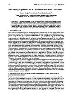
classification is consistent with the scene observed. C. Toward target detection in clutter In order to assess the performance of the algorithm for detecting hidden targets in vegetation, we use synthetic data to perform controlled experiments. We draw random points to produce a 5×5 m plate with a non null thickness and a 20 mtimes20 m point cloud. For each experiment, we varied the number of point for each elements: we reduce the number of point on the plate and increase the number of point for the clutter. The are able to achieve a 8 percent global error rate. Figure 7 shows one of the scene and classification result. The confusion matrix is presented in table I shows the number of prototype points correctly or incorrectly classified compared to the ground truth.
(a) XUV traverse Trajectory robot and LADAR acquisition positions
140
5
120
4.5
100 80
4 3.5
60
3
40
2.5 2
20 0 −700
Processing time vs nbr proto\point
5.5
duration (s)
relative northing (m)
160
−600
−500
−400 −300 −200 relative easting (m)
−100
0
(b) XUV path Fig. 5.
100
1.5 5
10
15 20 nbr proto_point (x1000)
25
30
(a) Raw data
(b) Classified data
(c) On-board processing time FITG experiment
Shortly after, we conducted an additional set of tests at GDRS facility in Westminster. The objective was to test a stand-alone version of the code, without the graphic interface, and to process and log the results. Figure 6 shows a twoclasse classification result. The scene is composed of two areas: 1) a rough terrain covered by tall grass unevenly distributed and bordered by tall trees, half left of Figure 6(a)/(b) and a parking lot with trees. Saliency features update and intermediate classication results were performed as the robot moved and the final classification result was stored. The
Fig. 7.
Synthetic data simulating a planar target hidden in vegetation
TABLE I C ONFUSION MATRIX FOR THE PLANE IN CLUTTER
Surface Point Line
Surface
Point
Line
1210 215 0
345 5605 0
3 35 0
(a) Top view Fig. 6.
(b) Side view
XUV results from Westminster test. In red/blue prototype points classified as surface/other.
V. S UMMARY AND FUTURE WORK
R EFERENCES
In this paper we presented a method to perform 3-D data segmentation for terrain classification in vegetated environment. Our method uses local point distribution statistics to produce saliency features that capture the surface-ness, curveness and point-ness of local area. We use statistical classification techniques to capture the variability of the scenes and the sensor characteristics (scanning pattern, range resolution, noise level). We fit a Gaussian mixture models to a training data set and use this parametric model to perform Bayesian classification. We implemented and tested our approach on a autonomous mobile robot, the GDRS XUV. We presented classification results from a static Z+F and Sick laser in addition to the results obtained on the XUV. With those examples we show the versatility and the limitations of our current method and implementation. Future work will focus on improving the processing time on reducing the classification error rate by dealing with border effects and isolated range measurements. We will also pay more attention to the formal numerical assessment of our method and to the problem of target hidden in vegetation. We also plan to implement opportunistic data processing of the ladar data, classifying data for obstacle detection only where the robot plans to drive.
[1] M. Hebert and N. Vandapel, “Terrain classification techniques from ladar data for autonomous navigation,” in Collaborative Technology Alliances Conference, May 2003. [2] J. Huang, A. Lee, and D.Mumford, “Statistics of range images,” in IEEE Conference on Computer Vision and Pattern Recognition, 2000, pp. I: 324–331. [3] J. Macedo, R. Manduchi, and L. Matthies, “Ladar-based discrimination of grass from obstacle for autonomous navigation,” in International Symposium on Experimental Robotics, 2000. [4] A. Castano and L. Matthies, “Foliage discimination using a rotating ladar,” in IEEE International Conference on Robotics and Automation, 2003. [5] G. Sithole and G. Vosselman, “Isprs comparison of filters,” ISPRS, Commission III, Working group 3, Tech. Rep., 2003. [6] A. Lacaze, K. Murphy, and M. Delgiorno, “Autonomous mobility for the demo iii experimental unmanned vehicles,” in Proceedings of the AUVSI 2002 Conference, 2002. [7] C. Wellington and A. Stentz, “Learning prediction of the load-bearing surface for autonomous rough-terrain navigation in vegetation,” in International Conference on Field and Service Robotics, 2003. [8] R. Duda, P. Hart, and D. Stork, Pattern Classification, 2nd ed. WileyInterscience, 2000. [9] G. Medioni, M. Lee, and C. Tang, A Computational Framework for Segmentation and Grouping. Elsevier, 2000. [10] J. Bilmes, “A gentle tutorial on the em algorithm and its application to parameter estimation for gaussian mixture and hidden markov models,” University of Berkeley, Tech. Rep. ICSI-TR-97-021, 1997. [11] J. Albus and al., “4d/rcs sensory processing and world modeling on the demo iii experimental unmanned ground vehicles,” in IEEE Internatinal Symposium on Intelligent Control, 2002. [12] ——, “4d/rcs version 2.0: A reference model architecture for unmanned vehicle system,” National Institute of Standards and Technology, Tech. Rep. NISTIR 6910, 2002. [13] D. Langer and al., “Imaging ladar for 3-d surveying and cad modeling of real world en vironments,” International Journal of Robotics Research, vol. 19, no. 11, 2000. [14] N. Vandapel, R. Donamukkala, and M. Hebert, “Experimental results in using aerial ladar data for mobile robot navigation,” in International Conference on Field and Service Robotics, 2003.
ACKNOWLEDGMENTS Prepared through collaborative participation in the Robotics Consortium sponsored by the U.S Army Research Laboratory under the Collaborative Technology Alliance Program, Cooperative Agreement DAAD19-01-209912. We would like to thanks General Dynamics Robotics System and specifically Bradley Stuart for his help with “laser3d” and the use of the autonomous vehicle.