Additional, thanks to Dan Sorin, David Woods, Shubhendu Mukherjee, Tim ... [8] F. Gabbay and A. Mendelson, âThe effect of instruction fetch bandwidth on value ...
Journal of Instruction-Level Parallelism 4 (2002) 1-27
Submitted 8/00; published 9/02
Using Statistical and Symbolic Simulation for Microprocessor Performance Evaluation Mark Oskin
OSKIN @ CS . WASHINGTON . EDU
Department of Computer Science and Engineering University of Washington Seattle, WA 98195 USA
Frederic T. Chong Matthew Farrens
CHONG @ CS . UCDAVIS . EDU FARRENS @ CS . UCDAVIS . EDU
Department of Computer Science University of California at Davis Davis, CA 95616 USA
Abstract As microprocessor designs continue to evolve, many optimizations reach a point of diminishing returns. We introduce HLS, a hybrid processor simulator which uses statistical models and symbolic execution to evaluate design alternatives. This simulation methodology enables quick and accurate generation of contour maps of the performance space spanned by design parameters. We validate the accuracy of HLS through correlation with existing cycle-by-cycle simulation techniques and current generation hardware. We demonstrate the power of HLS by exploring design spaces defined by two parameters: code properties and value prediction. These examples motivate how HLS can be used to set design goals and individual component performance targets.
1. Introduction In this paper, we introduce a new methodology of study for microprocessor design. This methodology involves statistical profiling of benchmarks using a conventional simulator, followed by the execution of a hybrid simulator that combines statistical models and symbolic execution. Using this simulation methodology, it is possible to explore changes in architectures and compilers that would be either impractical or impossible using conventional simulation techniques. We demonstrate that a statistical model of instruction and data streams, coupled with a structural simulation of instruction issue and functional units, can produce instructions per cycle (IPC) results that are within 5-7% of cycle-by-cycle simulation. Using this methodology, we are able to generate statistical contour maps of microprocessor design spaces. Many of these maps verify our intuitions. More significantly, they allow us to more firmly relate previously decoupled parameters, including: instruction fetch mechanisms, branch prediction, code generation, and value prediction. This work was originally presented in a short paper [1]. While the original version focused upon only one “average” application (perl) in the bulk of our design space explorations, this paper presents a broader range of data points for all design parameters examined. In addition to perl, xlisp and vortex are examined in depth – covering the extremes of instruction cache and branch predictor behavior in the SPEC95 suite. Novel material on the relationship of IPC variance and statistical accuracy is also presented. Finally, a more exhaustive set of results is included.
c 2002 AI Access Foundation and Morgan Kaufmann Publishers. All rights reserved.
O SKIN , C HONG & FARRENS
Execution Stage
Floating Point
Branch
Completion Unit (4 inst/cycle)
Dispatch Window (16 entry)
Integer
Fetch Unit (4 inst/cycle)
1111 0000 00000 000011111 1111 00000 11111 0000 1111 00000 11111 0000 1111 00000 11111 0000 1111 00000 L1 000011111 1111 00000 11111 00000 0000 1111 000011111 1111 00000 11111 I-Cache 000011111 1111 00000 00000 0000 1111 000011111 1111 00000 11111 0000 1111 11111 00000 0000 1111 00000 000011111 1111 00000 11111 0000 1111 Branch 00000 000011111 1111 11111 00000 Predictor 0000 1111 11111 00000 0000 1111 00000 11111 0000 1111 00000 000011111 1111 00000 11111 0000 1111 00000 11111 0000 1111 00000 L1 000011111 1111 00000 11111 0000 1111 00000 11111 0000 1111 00000 11111 000011111 1111 D-Cache 000000000 1111 00000 11111 0000 1111 00000 11111 0000 1111 11111 00000 0000 1111 00000 1111 000011111 Unified L2 Cache
Main Memory
1111 0000 0000 1111 0000 1111 0000 1111 0000 1111 0000 1111 0000 1111 0000 1111 0000 1111 0000 1111 0000 1111 0000 1111 0000 1111 0000 1111 0000 1111 0000 1111 0000 1111 0000 1111 0000 1111 0000 1111 0000 1111 0000 1111 0000 1111 0000 1111 0000 1111 0000 1111 0000 1111 0000 1111 0000 1111 0000 1111 1111 0000
Load / Store
Figure 1: Simulated Architecture
In the next section, we describe the HLS (High Level Simulator) simulator. Next in Section 3 we validate HLS against conventional simulation techniques. In Section 4, the HLS simulator is used to explore various architectural parameters. Then in Section 5, we discuss our results and summarize some of the potential pitfalls of this simulation technique. In Section 6, we discuss related work in this field. Finally, future work is discussed in Section 7, and Section 8 presents the conclusions.
2. HLS: A Statistical Simulator HLS is a hybrid simulator which uses statistical profiles of applications to model instruction and data streams. HLS takes as input a statistical profile of an application, dynamically generates a code base from the profile, and symbolically executes this statistical code on a superscalar microprocessor core. The use of statistical profiles greatly enhances flexibility and speed of simulation. For example, we can smoothly vary dynamic instruction distance or value predictability. This flexibility is only possible with a synthetic, rather than actual, code stream. Furthermore, HLS executes a statistical sample of instructions rather than an entire program, which dramatically decreases simulation time and enables a broader design space exploration which is not practical with conventional simulators. In this section, we describe the HLS simulator, focusing on the statistical profiles, method of simulated execution, and validation with conventional simulation techniques. 2.1 Architecture The key to the HLS approach lies in its mixture of statistical models and structural simulation. This mixture can be seen in Figure 1, where components of the simulator which use statistical models are shaded in gray. HLS does not simulate the precise order of instructions or memory accesses in 2
U SING S TATISTICAL AND S YMBOLIC S IMULATION FOR M ICROPROCESSOR P ERFORMANCE E VALUATION
Parameter Instruction fetch bandwidth Instruction dispatch bandwidth Dispatch window size Integer functional units Floating point functional units Load/Store functional units Branch units Pipeline stages (integer) Pipeline stages (floating point) Pipeline stages (load/store) Pipeline stages (branch) L1 I-cache access time (hit) L1 D-cache access time (hit) L2 cache access time (hit) Main memory access time (latency+transfer) Fetch unit stall penalty for branch mis-predict Fetch unit stall penalty for value mis-predict
Value 4 inst. 4 inst. 16 inst. 4 4 2 1 1 4 2 1 1 cycle 1 cycle 6 cycles 34 cycles 3 cycles 3 cycles
Table 1: Simulated Architecture configuration
a particular program. Rather, it uses a statistical profile of an application to generate a synthetic instruction stream. Cache behavior is also modeled with a statistical distribution. Once the instruction stream is generated, HLS symbolically issues and executes instructions much as a conventional simulator does. The structural model of the processor closely follows that of the SimpleScalar tool set [2], a widely used processor simulator. This structure, however, is general and configurable enough to allow us to model and validate against a MIPS R10K processor in Section 3.2. The overall system consists of a superscalar microprocessor, split L1 caches, a unified L2 cache, and a main memory. The processor supports out-of-order issue, dispatch and completion. It has five major pipeline stages: instruction fetch, dispatch, schedule, execute, and complete. The similarity to SimpleScalar is not a coincidence: the SimpleScalar tools are used to gather the statistical profile needed by HLS. We will also compare results from SimpleScalar and HLS to validate the hybrid approach. The simulator is fully programmable in terms of queue sizes and inter-pipeline stage bandwidth; however, the baseline architecture was chosen to match the baseline SimpleScalar architecture. The various configuration parameters are summarized in Table 1. 2.2 Statistical profiles In order to use the HLS simulator, an input profile of a real application must first be generated. Once the profile is generated, it is interpreted, a synthetic code sample is constructed, and this code is executed by the HLS simulator. Since HLS is probability-based, the process of execution is usually repeated several times in order to reduce the standard deviation of the observed IPC. This overall process flow is depicted in Figure 2. Statistical data collection of actual benchmarks is performed in the following manner: 3
O SKIN , C HONG & FARRENS
sim-outorder
Code
Binary
Stat profile
Stat-binary
HLS
sim-stat
Figure 2: Simulation process
Value Basic block size (�) Basic block size (� ) Integer Instructions FP Instructions Load Instructions Store Instructions Branch Instructions Branch Predictability L1 I-cache hit rate L1 D-cache hit rate L2 cache hit rate
perl 5.21 3.63 30% 1% 31% 18% 19% 91.4% 96.4% 99.9% 99.9%
compress 4.69 4.91 42%