Parallel EM Learning for SymbolicStatistical Models Yusuke Izumi
Department of Computer Science, Graduate School of Information Science and Engineering, Tokyo Institute of Technology, Japan
[email protected]
Yoshitaka Kameya
(affiliation as previous author)
[email protected]
Taisuke Sato
(affiliation as previous author)
[email protected]
keywords: parallel EM algorithm, symbolic-statistical models, PRISM, distributed parallel computing Summary EM learning, i.e. parameter learning for probabilistic models using the EM algorithm, requires a larger amount of time and memory space as data size increases. One way to cope with this problem is to take advantage of the power of parallel computing. In this paper, we introduce a data-parallel algorithm for EM learning applicable to the probabilistic models represented by PRISM, a programming language for symbolic-statistical modeling. We also present the results of two learning experiments, one for HMMs with randomly-generated data and the other for PCFGs with Penn Treebank III. The results show good performance of the proposed algorithm in terms of the speed-up of our algorithm up to 33 processors for HMMs, as well as in terms of memory space utilization up to nearly 30 gigabytes in total for PCFGs with 21 computational nodes.
1. Introduction Probabilistic modeling provides a powerful way to deal with uncertain information. One of the basic tasks in probabilistic modeling is parameter learning, and the EM (expectation-maximization) algorithm [Dempster 77] has been widely used for that purpose. While various methods of EM learning have been proposed for specific models, PRISM (programming in statistical modeling) [Sato 01] has been developed to provide a unified way of probabilistic modeling and EM learning. PRISM is based on distribution semantics, which is a probabilistic extension of the least model semantics in logic programming [Lloyd 84]. Each PRISM program defines a probability distribution for symbolic-statistical models, which refer to models represented by symbolic objects such as HMMs (hidden Markov models), PCFGs (probabilistic context-free grammars), and discrete Bayesian networks. In addition, the PRISM system provides general-purpose parameter learning routines based on the gEM (graphical EM) algorithm [Kameya 00]. In general, larger data sets lead to more statically
reliable results. Fortunately, thanks to progress in information technology including the Internet, it becomes more and more feasible to use a large amount of data. To take advantage of this opportunity for EM learning, we need a powerful computing system. The objective of this paper is to utilize the power of parallel computing for EM learning. There are parallel EM algorithms for several problems [L´opez-deTeruel 99, Zhang 00, Kruengkrai 02], but they are problem-specific, not applicable to wide range of symbolic-statistical models. Furthermore, they implicitly assume parameter sets to be known in advance, but PRISM allows parameter sets to be determined during computation dependently on the given data. In this paper, we propose a data-parallel version of the gEM algorithm called the pgEM (parallel gEM) algorithm, which is applicable to any probabilistic models on which the gEM algorithm works. In what follows, we explain PRISM and the gEM algorithm in Chapter 2, describe the pgEM algorithm in Chapter 3, show experimental results in Chapter 4, and give conclusion in Chapter 5.
a, b a, b
s0
s1
a, b
a, b
target(hmm/1).
% we observe hmm(_).
values(init ,[s0,s1]). % initial state values(out(_),[a,b]). % output values(tr(_) ,[s0,s1]). % transition hmm(Xs) :msw(init,Q), hmm(1,Q,Xs).
% generation: % choose initial state % go into loop
hmm(T,_,[]) :- T>3,!. hmm(T,Q,[X|Xs]) :msw(out(Q),X), msw(tr(Q),Q1), T1 is T+1, hmm(T1,Q1,Xs).
% stop the loop % loop: (until T > 3) % output symbol % transit to next state % turn to next step % repeat(by recursion)
hmm([a,b,a]) ↔ hmm(1,s0,[a,b,a]) ∧ msw(init,s0) ∨ hmm(1,s1,[a,b,a]) ∧ msw(init,s1) hmm(1,s0,[a,b,a]) ↔ hmm(2,s0,[b,a])† ∧ msw(out(s0),a) ∧ msw(tr(s0),s0) ∨ hmm(2,s1,[b,a]) ∧ msw(out(s0),a) ∧ msw(tr(s0),s1) hmm(1,s1,[a,b,a]) ↔ hmm(2,s0,[b,a])† ∧ msw(out(s1),a) ∧ msw(tr(s1),s0) ∨ hmm(2,s1,[b,a]) ∧ msw(out(s1),a) ∧ msw(tr(s1),s1) hmm(2,s0,[b,a])‡ ↔ hmm(3,s0,[a]) ∧ msw(out(s0),b) ∧ msw(tr(s0),s0) ∨ hmm(3,s1,[a]) ∧ msw(out(s0),b) ∧ msw(tr(s0),s1) hmm(2,s1,[b,a]) ↔ hmm(3,s0,[a]) ∧ msw(out(s1),b) ∧ msw(tr(s1),s0) ∨ hmm(3,s1,[a]) ∧ msw(out(s1),b) ∧ msw(tr(s1),s1) hmm(3,s0,[a]) ↔ msw(out(s0),a) ∧ msw(tr(s0),s0) ∨ msw(out(s0),a) ∧ msw(tr(s0),s1) hmm(3,s1,[a]) ↔ msw(out(s1),a) ∧ msw(tr(s1),s0) ∨ msw(out(s1),a) ∧ msw(tr(s1),s1)
Fig. 1 HMM (above) and PRISM program (below). Fig. 2 An explanation graph for hmm([a,b,a]).
2. Preliminary 2・1 PRISM Informally PRISM is a Prolog extended with special predicates for probabilistic modeling. Here, we briefly explain the PRISM language with an example program shown in Figure 1.∗1 This program represents an HMM that has two states {s0, s1} and outputs a symbol either a or b at each state. target(hmm/1)∗2 declares that we observe events represented by atoms of the form hmm(·). msw/2 is a special predicate that denotes a probabilistic choice. Specifically, a ground atom msw(i,v) indicates that a discrete random variable i takes a value v from the set Vi of possible values, where Vi is specified by a special predicate values/2 (e.g. Vtr(·) = {s0, s1}). Hereafter, we refer to a random variable i as a switch, and a ground atom msw(i,v) as a switch instance, following the terms in the current PRISM implementation. Each switch i is regarded as an independent and identically distributed random variable. A probability distribution defined by a PRISM program is specified by parameters of switch instances, each of which gives the probability θi,v of a switch i P taking a value v in msw/2 ( v∈Vi θi,v = 1). Parameters may be set by users, or by estimation from data (or observed goals) as we discuss next. ∗1 The reader is referred to [Sato 01] for a detailed description. ∗2 p/n denotes a predicate p of arity n.
2・2 EM Learning for PRISM Programs The EM algorithm is a well-known class of iterative algorithms for ML (maximum likelihood) estimation of statistical parameters from data with hidden information. For example, in the HMM program above, the state at each step is hidden from observed goals hmm(·). Specifically for HMMs, parameter estimation can be done by an efficient EM algorithm known as the Baum-Welch or the forward-backward algorithm [Rabiner 89]. On the other hand, PRISM is not limited to HMMs, so we need a more general EM algorithm. At the same time, though, the algorithm should be comparable in terms of efficiency with specialized algorithms such as the Baum-Welch algorithm. Previous works (e.g. [Sato 01]) present a two-stage method that fulfills such requirements: tabled search and the gEM algorithm. Tabled search finds logical explanations for given goals with tabling (i.e. memoizing) intermediate subgoals and reusing them for later calls.∗3 The reuse makes the derivation paths for different calls of the same subgoal shared. After the search, the derivation paths are translated into And-Or graphs called explanation graphs. The gEM algorithm then runs on these explanation graphs to estimate parameters θi,v . Figure 2 shows an explanation graph for a goal hmm([a,b,a]). Note that two distinct calls marked with † in the figure refer to the ∗3 The current implementation is based on linear tabling [Zhou 03].
same subgoal marked with ‡, which indicates structure sharing occurs here. Let G = hG1 , . . . , GT i be a series of observed goals. Then an explanation graph for each Gt (1 ≤ t ≤ T ) (t) (t) is formulated by Tt = hτ0 , . . . , τKt i, an ordered set ˜ (t) ) (1 ≤ k ≤ Kt ), of distinct tabled subgoals, and ψ(τ
#0 (Master ) subtask assigned next
work pool (queue of subtasks )
k
(t) (t) a disjunction of S˜k,j (1 ≤ j ≤ mk ) where each S˜k,j is a conjunction of subgoals and switch instances. It (t) must hold that τ0 = Gt and that τk does not appear 0 ˜ (t) in ψ(τ 0 ) for any k ≤ k . The latter condition implies
#1 (Slave)
#2 (Slave)
#3 (Slave)
Fig. 3 The work pool method.
k
that subgoal calls should be acyclic. This acyclicity allows dynamic programming in the gEM algorithm. The gEM algorithm computes the inside probability P[t, τ ] of each subgoal τ ∈ Tt from the end to the beginning of the sequence Tt , then the outside probability Q[t, τ ] as well as expected counts η[t, i, v] of switch instances in the goal Gt from the beginning to the end.∗4 The expected counts are summed up over goals to obtain the total expected counts η[i, v] (E-step), then the parameters θi,v are updated using these values of η[i, v] (M-step). These steps are iterated unPT til convergence of log likelihood λ = t=1 log P[t, Gt ]. The gEM algorithm runs in time and space linear to PT PKt Pmk ¯¯ ˜(t) ¯¯ ξ = t=1 k=1 j=1 Sk,j , the total size of explanation graphs. It has been shown that the gEM algorithm, despite its generality, has the same time complexity as some widely-used EM algorithms designed for specific models including the Baum-Welch algorithm for HMMs [Sato 01]. However, the algorithm still requires time and space proportional to T , the number of observed goals, thus there may be cases in which the gEM algorithm on a single computer does not work. In the next chapter, we introduce a new learning algorithm based the gEM algorithm for parallel computing.
3. Parallel EM Learning 3・1 Distributing Subtasks The task for parameter estimation described in the previous chapter can be naturally divided into subtasks, each associated with a single observed goal. Tabled search obviously can be performed independently for each goal.∗5 The inside and outside probabilities are also computed separately for each goal. ∗4 Roughly speaking, the inside probability of a subgoal τ is the probability of τ being true, and the outside probability of a subgoal τ is the probability that all subgoals preceding and following τ are true. ∗5 PRISM programs are assumed to be shared among all processors.
The only values that need to be shared among processors are the log likelihood λ and the total expected counts η[i, v] of switch instances.∗6 While our strategy for task division is simple, we need to be careful about distributing subtasks and sharing the values λ and η[i, v] for efficient computation. We discuss how to distribute subtasks in this section and how to share the values in the next section. In distributing observed goals, we should respect load balancing for parallel efficiency. It is not appropriate, for example, to simply assign the same number of observed goals to each processor, since search spaces and sizes of explanation graphs may vary among goals. On the other hand, there is no generic way to predict search spaces or sizes of explanation graphs without performing actual search. Hence we apply a work pool method [Wilkinson 99], which is a well-known method for dynamic assignment. This method is based on a master-slave model, where one processor works as a master process and the others as slave processes. The master process first assigns a single subtask to each slave process. Then each slave process executes the assigned subtask. After completion of the subtask, a slave process tells the result to the master process and receives another subtask. The entire task ends when all subtasks are executed by slave processes. Figure 3 illustrates how the work pool method works. This usually balances the load among slave processes as long as the number of subtasks is sufficiently large. Strictly speaking, we should consider the load balancing for both tabled search and the gEM algorithm. In this respect, it is not practical to alter assignments of observed goals for tabled search and for the gEM algorithm because it requires exchange of large data structure for explanation graphs. Fortunately, however, it is expected that the size of an extracted expla∗6 The parameters θi,v can be obtained from η[i, v].
nation graph is roughly proportional to time required for search, and it has been proved that time complexity of the gEM algorithm is proportional to the size of explanation graph. So we can assign goals simply depending on time consumed for tabled search, expecting the load to be balanced in practice. 3・2 Sharing the Values As stated above, the log likelihood λ and the total expected counts η[i, v] of switch instances need to be shared. Since the log likelihood λ is given by the sum of the log inside probabilities of all observed goals, the value can be easily shared as follows. Each processor p computes the local log likelihood λp , the sum of the log inside probabilities of observed goals assigned to the processor p. All processors then exchange the values of λp each other and compute the P log likelihood λ = p λp . The total expected counts η[i, v] also can be shared in a similar way, but there is a difficulty: the set of used switch instances may differ among processors. PRISM programs may have switches with variables like tr(_) in the HMM program in Figure 1, which introduce (potentially) an infinite number of switch instances. Tabled search reduces infinite switch instances to finite ones by seeking ones that actually occur in the logical explanation for the observed goals, as seen from Figure 2. The sets of occurring switch instances can vary among the observed goals, thus processors may have different sets of switch instances. The exchange method for the total expected counts η[i, v] need to adapt this situation. One way may be to exchange a pair of the name and the expected count for every switch instance, but it can be too inefficient because names of switch instances become sometimes fairly long. Our proposal is to exchange the expected counts using linear arrays of the same layout. After tabled search, each slave process p sorts switches whose instances occur on the processor p, in order of their names, then sends the resultant sequence Ip to the master process. After receiving the sequences from all slave processes, the master process merges them to obtain the entire sequence I of switches. Then the master process enumerates every switch instance, i.e. every pair of i ∈ I and v ∈ Vi , in order of the sequence I to determine the starting index of each switch in the array for exchange. Finally, the master process sends the starting indices of switches in Ip as well as the size of the entire array. With the starting indices and the entire size, and the ordering of values
v ∈ Vi given by values/2 predicates, an array of the same layout is built on each processor. Figure 4 illustrates this procedure. Each array element contain PTp ηp [i, v] = t=1 η[t, i, v], the local expected count of a switch instance msw(i,v) on the processor p. Labels ‘?’ on array elements indicate absence of the corresponding switch instances, and so these elements should contain zero. Each symbol ‘+’ in the figure denotes some non-negative value. 3・3 The pgEM Algorithm The parallel version of the gEM algorithm is shown in Figure 5. This is the same as the original algorithm except for sharing of the log likelihood λ and the total expected counts η[i, v]. With P processors, this algorithm is expected to run roughly (P − 1) times faster than the original algorithm, as long as the load is balanced, since observed goals are distributed over (P − 1) slave processes.
4. Experiments We conducted two learning experiments to evaluate the performance of the pgEM algorithm: HMMs with randomly-generated data and PCFGs with Penn Treebank III,∗7 a real-world corpus. Our implementation is made using MPI (message passing interface) [Gropp 99] as a library for parallelization, and based on beta versions of PRISM 1.10. Both experiments were carried out with up to 21 nodes each of which has dual Athlon MP 1900+ and 2GB RAM. These nodes are connected via Gbps ethernet. 4・1 HMMs The first experiment was conducted using the HMM program shown in Figure 1 but the string length was set to 20.∗8 We generated from 2,500 to 20,000 samples as a data set using parameters shown in Table 1. We prepared five sets for each size. Figure 6 shows the speed-up ratio to the original system (running with a single processor) in terms of average learning time when one of dual processors is used on each node. A dashed line indicates (P − 1) switch init tr(s0) tr(s1)
s0 0.9 0.2 0.8
s1 0.1 0.8 0.2
switch out(s0) out(s1)
a 0.5 0.6
b 0.5 0.4
Table 1 Sampling parameters. ∗7 http://www.ldc.upenn.edu/. ∗8 The program in Figure 1 is for the length of three.
ha, 0i ha, 1i hb, xi hb, yi hb, zi hc, 0i hc, 1i hd, 0i hd, 1i
#0 (Master )
switch index
a 0
b 2
c 5
d 7
0
0
0
0
0
0
0
0
0
0
1
2
3
4
5
6
7
8
ha, 0i ha, 1i
#1 (Slave)
switch index
a 0
c 5
#2 (Slave)
switch index
b 2
c 5
#3 (Slave)
switch index
a 0
b 2
d 7 d 7
+
+
?
?
0
0
?
?
?
0
0
0
+
hc, 0i hc, 1i hd, 0i hd, 1i
+
+
+
+
η1
hb, xi hb, yi hb, zi hc, 0i hc, 1i hd, 0i hd, 1i
+
+
+
ha, 0i ha, 1i hb, xi hb, yi hb, zi
+
η0
+
+
+
+
+
+
+
?
?
?
?
0
0
0
0
η2
η3
Fig. 4 Exchanging expected counts. Va = Vc = Vd = {0, 1}, Vb = {x, y, z}.
where P is the number of processors. Figure 6 shows that the greater speed-up ratio is realized as the number of samples increases. This is probably because the samples (i.e. observed goals) are distributed in a more balancing way when more samples are given. In addition, super-linear speed-up is observed in the cases of 10,000 and 20,000 samples. For example, when the number of samples is 20,000, average learning time of 1,852 seconds with a single processor was reduced to 54 seconds with 21 processors, that is, the parallel version runs 34 times faster. Our understanding is that this super linearity is caused by heavy use of memory space as shown in Figure 7 affecting efficiency on memory access, e.g. CPU cache.∗9 We also tried using both of dual processors. The results are shown in Figure 8. Since some resources including memory are shared by each pair of processors, the speed-up ratio is not so high as that shown in Figure 6. However, Figure 8 shows the parallel scalability of our algorithm up to 33 processors in the case of 20,000 samples. 4・2 PCFGs PCFGs are a probabilistic extension of context-free grammars widely used in statistical natural language processing. Each production rule A → α∗10 in a PCFG P has a probability θA→α such that α θA→α = 1 holds for every non-terminal A. Figure 9 shows a PRISM program for PCFGs. A predicate pcfg(A,L0 ,L1 ) where L0 = [wi ,...,wN ] and L1 = [wj+1 ,...,wN ] (wk denotes a terminal, namely a word) means that the substring L0 − L1 = [wi ,...,wj ] is governed by a non-terminal A. A probabilistic event that a rule A → α is chosen for a non-terminal A is represented by msw(A,n), where n is the identification number of the rule and α is fetched by rhs(n,α). An auxiliary ∗9 Each processor has 128KB of L1 cache (64KB each for data and instructions) and 256KB of L2 cache. ∗10 Symbols α, β, . . . denote sequences of terminals and nonterminals.
predicate preq/2 is introduced for pruning on tabled search by calling first(A,w), which means there is a series of projections of production rules from a non-terminal A to generate a string beginning with a terminal w. Actual ground terms of first/2 are precomputed and given as part of the program. Lastly, proj/3 attempts projection. The learning experiment was carried out as follows. We first randomly picked up from 100 to 1,000 sentences of length ≤ 40 from articles of Wall Street Journal (43,804 sentences) with the corresponding parse trees. Words in the sentences were replaced with their POS (part-of-speech) tags. We prepared three sets of sentences for each data size. Then we extracted CFG rules from those parse trees in a straightforward way.∗11 Characteristics of the extracted rules are shown in Table 2. Under these settings, we conducted estimation of parameters θA→α from the picked-up sentences (with smoothing for faster convergence) using one processor on each node. This is a challenging task because the number of possible parse trees for a single sentence can be 2.9 × 1048 at the maximum. Table 3 and Table 4 show the range of learning time and average memory space consumed on each slave process respectively. Bars indicate that the program doesn’t work due to the memory limit under the corresponding conditions.∗12 A larger number of nodes provide a larger memory space and hence enable use of more sentences on learning, though memory usage is not in linear to the number of sentences owing to increase in the number of extracted rules. The results also show that our implementation makes it possible to use nearly 30 gigabytes in total of memory space. ∗11 To produce more likely suitable rule sets, we added an auxiliary attribute gap as in [Collins 97]. This attribute indicate that a syntactic element has a gap caused by whmovement, e.g. ◦ in a noun phrase “a person who ◦ saw you yesterday”. ∗12 B-Prolog, the base system of PRISM, has limit of roughly one gigabyte for its working areas in 32-bit environments, though PRISM may allocate extra memory area beyond this limit.
˜ T) procedure Get-Inside-Probs(ψ, begin for t := 1 to T do begin
35
(t)
(t)
P[t, τk ] := 0; ˜ (t) ) do begin foreach S˜ ∈ ψ(τ k Let S˜ = {A1 , A2 , . . . , A ˜ };
25 Speed-up
Put Gt = τ0 ; for k := Kt downto 0 do begin
|S|
15
5 0 1
5
9 13 Number of Processors
k
else (t) ˜ (t) ˜ R[t, τk , S] = R[t, τk , S] · P[t, Al ] ˜ end (* foreach S *) end (* for k *) end (* for t *) end
(t)
Let Gt = τ0 ; := 1; (t)
for k := 1 to Kt do Q[t, τk ] := 0; foreach i ∈ I, v ∈ Vi do η[t, i, v] := 0; for k := 0 to Kt do ˜ (t) ) do begin foreach S˜ ∈ ψ(τ k ˜ Let S = {A1 , A2 , . . . , A ˜ };
21
250 #samples = 2500 #samples = 5000 #samples = 10000 #samples = 20000
200
150
100
50
0 1
|S|
˜ do for l := 1 to |S| if Al = msw(i,v) then η[t, i, v] := η[t, i, v] +
17
Fig. 6 Speed-up for HMMs.
Memory Usage in Megabytes
˜ T) procedure Get-Expectation(ψ, begin for t := 1 to T do begin (t) Q[t, τ0 ]
20
10
(t) ˜ R[t, τk , S] := 1; ˜ do for l := 1 to |S| if Al = msw(i,v) then (t) ˜ (t) ˜ R[t, τ , S] = R[t, τ , S] · θi,v k
#samples = 2500 #samples = 5000 #samples = 10000 #samples = 20000
30
5
9 13 Number of Processors
17
21
Fig. 7 Memory usage for HMMs on each slave processor.
(t) (t) ˜ Q[t, τk ] · R[t, τk , S]/P[t, Gt ]
else Q[t, Al ] := Q[t, Al ] +
45
(t) (t) ˜ Q[t, τk ] · R[t, τk , S]/P[t, Al ] ˜ end (* foreach S *) end (* for t *) end
Fig. 5 The pgEM algorithm.
35 30 Speed-up
˜ T) procedure Parallel-Learn-gEM (ψ, begin Initialize and broadcast θ at the master process; ˜ ); Get-Inside-Probs(ψ,T PTp λp := t=1 ln P[t, Gt ]; P Share λ := p λp ; repeat λold := λ; ˜ T ); Get-Expectations(ψ, foreach i ∈ I, v ∈ Vi do PTp ηp [i, v] := t=1 ln η[t, i, v]; P Share η[i, v] := p ηp [i, v] for all hi, vi; (* see Section 3・2 *) foreach i ∈ I, v ∈ V do i P θi,v := η[i, v]/ v0 ∈Vi η[i, v 0 ]; ˜ T ); Get-Inside-Probs(ψ, PTp λp := t=1 ln P[t, Gt ]; P Share λ := p λp until λ − λold < ε (* loop until convergence *) end
#samples = 2500 #samples = 5000 #samples = 10000 #samples = 20000
40
25 20 15 10 5 0 1
5
9
13
17 21 25 Number of Processors
33
41
Fig. 8 Speed-up for HMMs with use of dual processors.
Size
#rules
#T
#NT
100 200 300 450 600 800 1000
1333 – 1751 2005 – 3055 3924 – 4440 5930 – 7297 5442 – 6972 6753 – 7391 11294–12351
35–40 40–41 40–43 42–44 42–45 44–44 43–45
23–28 28–32 27–33 32–33 34–34 34–34 35–35
#parse trees (median) 6.6e08–1.9e10 7.8e09–1.5e12 1.3e11–5.3e16 7.2e16–5.7e18 4.3e15–5.7e19 1.3e17–1.2e19 1.4e20–4.4e22
#parse trees (max.) 2.3e18–3.7e20 1.5e21–8.0e30 1.2e29–7.4e36 5.6e35–7.6e39 4.0e37–6.0e43 2.9e39–1.1e43 1.1e45–2.9e48
Table 2 Rule characteristics. T and NT denote terminals and non-terminals respectively. 6.6e08 denotes 6.6×10⁸ .
target(sent/1). sent(L) :- start(S),!,pcfg(S,L,[]). pcfg(LHS,L0,L1) :( terminal(LHS) -> L0 = [LHS|L1] ; msw(LHS,N), rhs(N,RHS), preq(RHS,L0), proj(RHS,L0,L1) ). preq([],_). preq([X|_],[Y|_]) :- first(X,Y),!. preq([X|_],[Y|_]) :- X == Y,!. proj([],L,L). proj([X|Xs],L0,L1) :pcfg(X,L0,L2), preq(Xs,L2), proj(Xs,L2,L1). Fig. 9 A PCFG program.
Size 1 node 3 nodes 5 nodes 11 nodes 100 22 – 44 11 – 24 6 – 12 3 – 5 200 147 – 220 76 – 143 36 – 58 15 – 27 300 — 363 – 596 134 – 237 74 – 115 450 — — 389 – 939 163 – 392 — — — 240 – 650 600 800 — — — 579 –1313 1000 — — — —
21 nodes 2 – 3 8 – 25 42 – 56 80 – 198 148 – 390 359 – 801 696 –1547
Table 3 Learning time for PCFGs (in seconds). Size 1 node 3 nodes 5 nodes 100 151 – 260 54 – 93 34 – 58 200 645 – 776 221 – 265 136 – 163 — 574 – 868 348 – 541 300 450 — — 951 –1217 600 — — — — — — 800 1000 — — —
11 nodes 18 – 29 66 – 78 167 – 248 450 – 619 656 –1072 1052–1265 —
21 nodes 12 – 17 36 – 44 90 – 133 238 – 329 350 – 594 582 – 713 1032–1417
Table 4 Memory usage for PCFGs (in megabytes).
It is advantage of parallel computing that such a huge memory space is available.
5. Related Work and Conclusion In this paper, we have presented the pgEM algorithm, a data-parallel algorithm for EM learning of symbolic-statistical models. We have also empirically demonstrated the scalability of the pgEM algorithm for HMMs and PCFGs. Use of multiple computers reduces computation time as well as extends memory space available for learning, and hence makes learning from data sets of much greater size feasible. There are problem-specific parallel EM algorithms for computer vision [L´ opez-de-Teruel 99], general clustering [Zhang 00], and document classification [Kruengkrai 02]. They are all data-parallel algorithms as our algorithm is, but the former two algorithms are specialized for finite mixture models and the latter
one for naive Bayes models. [L´opez-de-Teruel 99] and [Kruengkrai 02] do not mention how to assign subtasks to processors unlike us in Section 3・1, and seem to assign in a static way (maybe by the number of samples or by hand). [Zhang 00] allows dynamic load balancing by reassignment of subtasks. Reassignment is basically a good idea, but only applicable to algorithms for specific probabilistic models. A more notable difference between these algorithms and ours is the handling of parameter sets. The existing algorithms are applicable only for probabilistic models in which parameter sets can be determined beforehand. On the other hand, our algorithm allows parameter sets to be dynamically determined from data (observed goals) during computation by the mechanism stated in Section 3・2. This gives us greater flexibility in probabilistic modeling. For example, in lexicalized PCFGs [Collins 97], a linguistically motivated extension of PCFGs, each non-terminal is associated with a word or a POS tag. Therefore parameter sets for a lexicalized PCFG are not determined until sentences are given. Currently, we are planning to conduct learning experiments with lexicalized PCFGs. Acknowledgments This research is supported by the 21st Century COE Program “Framework for Systematization and Application of Large-scale Knowledge Resources”. We are also grateful to the administrators and users of the 21COE-LKR grid computer for their cooperation on our experiments. Thanks to Neng-Fa Zhou for his help with our implementation and Kenichi Kurihara for comments on our experiments.
♦ References ♦ [Collins 97] Collins, M.: Three Generative, Lexicalised Models for Statistical Parsing, in Proceedings of the 35th annual meeting on Association for Computational Linguistics, pp. 16–23 (1997) [Dempster 77] Dempster, A. P., Laird, N. M., and Rubin, D. B.: Maximum Likelihood from Incomplete Data via the EM Algorithm, Royal Statistical Society, Vol. 39, No. 1, pp. 1–38 (1977) [Gropp 99] Gropp, W., Lusk, E., and Skjellum, A.: Using MPI: Portable Parallel Programming with the MessagePassing Interface, MIT Press, 2nd edition (1999) [Kameya 00] Kameya, Y. and Sato, T.: Efficient EM learning with tabulation for parameterized logic programs, in Proceedings of the 1st International Conference on Computational Logic, Vol. 1861 of LNAI, pp. 269–294 (2000) [Kruengkrai 02] Kruengkrai, C. and Jarukulchai, C.: A Parallel Learning Algorithm for Text Classification, in Proceedings of the eighth ACM SIGKDD international conference on Knowledge discovery and data mining, pp. 201–206 (2002)
[Lloyd 84] Lloyd, J. W.: Foundations of Logic Programming, Springer-Verlag (1984) [L´ opez-de-Teruel 99] L´ opez-de-Teruel, P. E., Garc´ıa, J. M., and Acacio, M.: The Parallel EM Algorithm and its Applications in Computer Vision, in Parallel and Distributed Processing Techniques and Applications, pp. 571–578 (1999) [Rabiner 89] Rabiner, L. R.: A Tutorial on Hidden Markov Models and Selected Applications in Speech Recognition, in Proceedings of the IEEE, Vol. 77, pp. 257–286 (1989) [Sato 01] Sato, T. and Kameya, Y.: Parameter Learning of Logic Programs for Symbolic-statistical Modeling, Journal of Artificial Intelligence Research, Vol. 15, pp. 391–454 (2001) [Wilkinson 99] Wilkinson, B. and Allen, M.: Parallel Programming: Techniques and Applications Using Networked Workstations and Parallel Computers, Prentice Hall (1999) [Zhang 00] Zhang, B., Hsu, M., and Forman, G.: Accurate Recasting of Parameter Estimation Algorithms using Sufficient Statistics for Efficient Parallel Speed-up, in Proceedings of the 4th European Conference on Principles and Practice of Knowledge Discovery in Databases, pp. 243–254 (2000) [Zhou 03] Zhou, N.-F. and Sato, T.: Efficient Fixpoint Computation in Linear Tabling, in Proceedings of the 5th ACM-SIGPLAN International Conference on Principles and Practice of Declarative Programming, pp. 275–283 (2003)