Jun 18, 2008 - the solution of fully populated nonsymmetric matrices, the computer ... less than 1 min using a standard Dell Precision M70 laptop computer.
Using the Complex Polynomial Method with Mathematica to Model Problems Involving the Laplace and Poisson Equations A. C. Poler,1 A. W. Bohannon,1 S. J. Schowalter,1 T. V. Hromadka II2 1 United States Military Academy, West Point, New York 10996 2
Department of Mathematical Sciences, United States Military Academy, West Point, New York 10996
Received 26 November 2007; accepted 3 January 2008 Published online 18 June 2008 in Wiley InterScience (www.interscience.wiley.com). DOI 10.1002/num.20365
The complex polynomial method variant of the well-known complex variable boundary element method (CVBEM) is reexamined in its utility in solving Partial Differential Equations (PDE) of the Poisson and Laplace type. Because the CVBEM was recently extended to three and higher dimensions, the use of complex polynomials to solve higher dimension PDE becomes apparent and therefore the advantages afforded by the use of complex polynomials can be brought to focus on higher dimension problems. Because complex polynomials involve use of computational algorithms that require high accuracy in numerical precision, including the solution of fully populated nonsymmetric matrices, the computer program Mathematica is evaluated for use as the underlying computational engine. Furthermore, Mathematica is evaluated for its internal highaccuracy computational features and algorithms, including ease of program setup. In this research, the new program is found to provide at least a 5-fold increase in complex polynomial degree utilization (from degree 10 to degree 50), with computational speed less than was involved in the original degree 10 approximation of Hromadka and Guymon [ASCE J Hydraulic Eng 110 (1984), 329–339], and with exceptional computational accuracy and reporting features. The Mathematica program is quite small and is provided to the reader as freeware and can be obtained from the first author. © 2008 Wiley Periodicals, Inc. Numer Methods Partial Differential Eq 25: 657–667, 2009
Keywords: complex polynomials; Laplace’s equation; numerical methods; Dirichlet problem
I. INTRODUCTION
The complex variable boundary element method or CVBEM is a numerical technique for solving multidimensional problems involving the Poisson equation or the more standard Laplace equation with various types of boundary conditions, sinks, or sources, among other auxiliary capabilities. The intent of the numerical approach is to either collocate or employ an Lp norm to minimize the Correspondence to: A. C. Poler, United States Military Academy, West Point, New York 10996 (e-mail: andrewpoler@ gmail.com) © 2008 Wiley Periodicals, Inc.
658
POLER ET AL.
error in the approximate solution of the governing partial differential equation (PDE) and boundary conditions. Because the bases used contain only elements that solve the Laplace equation, the PDE is solved exactly in the problem domain, and the error on the boundary is minimized in the selected Lp norm, usually the common Lp with p = 2, or “least square error” minimization. By the Maximum Modulus Principle, the supremum norm error (used in collocation) on the problem boundary maximizes the modeling error throughout the problem domain. Further, the resulting approximation function exists not only inside the problem domain and on the boundary, but also outside of the domain, and so an “approximate boundary” is readily developed where the resulting approximation function meets the prescribed boundary condition values, which is useful in assessing the goodness of fit to the problem boundary conditions. In application, the closeness of fit between the approximate boundary and the actual problem boundary gives a measure of the goodness of the numerical approximation function in solving the boundary value problem. Details about this numerical approach, application to problems in various fields of study, and the theoretical development, can be found in Hromadka and Whitley [1] and Hromadka [2]. Complex polynomials have the advantage that they are analytic throughout the entire space (extension of the CVBEM approach to three and higher dimensions is given in Hromadka [2]) and, therefore, the resulting approximation functions are readily evaluated outside of the problem domain. Another advantage in using complex polynomials is that a self-generation algorithm can be developed to produce successively higher degree complex polynomials which can then be resolved into real function components that are individually harmonic functions. An issue with this complex polynomial approach, however, is that large basis function set size (i.e., higher dimension of the basis) involves computations that require a high level of accuracy to be useful, and the solutions demonstrate instability outside of the problem boundary. To satisfy the high accuracy computational needs of complex polynomials, the computer program Mathematica is used to develop a program that implements the Complex Polynomial Method variant of the CVBEM. The resulting application provided more than a 5-fold increase in computational capacity in the number of complex polynomials accommodated. For example, Hromadka and Guymon [3] reported use of up to 10 complex polynomials. In comparison, the current research effort used degree 50 complex polynomials and it was apparent that use of higher degree polynomials may be used. Furthermore, the time needed to solve the degree 50 complex polynomial approximations was less than 1 min using a standard Dell Precision M70 laptop computer. Finally, Mathematica can be programmed directly to take advantage of its high-accuracy internal computational and algorithmic features, rather than needing auxiliary programs to perform relevant computational tasks such as matrix setup and matrix solving. Mathematica also provides a wide array of means by which to display computational results.
II. LITERATURE REVIEW
A special issue of the Journal of Engineering Analysis with Boundary Elements (Vol. 30, No. 12, December 2006) provides a recent review of activity and advances in the CVBEM. Not found in that special issue is discussion involving the Complex Polynomial Method variant of the CVBEM, and so a brief background is provided. The work of Hromadka and Guymon [3] developed the complex polynomial variant of the CVBEM and successfully applied the technique to a number of practical engineering and physics problems. Because of the computational advantages afforded by other basis functions, such as the product of linear complex polynomials with complex logarithmic functions defined according to a nodal discretization of the problem boundary (e.g., Hromadka and Lai [4] and Hromadka Numerical Methods for Partial Differential Equations DOI 10.1002/num
COMPLEX POLYNOMIAL METHOD WITH MATHEMATICA
659
and Whitley [1]), the CVBEM development focused on that particular choice of family of basis functions. In 2002, the two-dimensional limitation of the CVBEM was broken by the extension of the CVBEM to arbitrary three and higher dimensions for the solution of the Poisson and Laplace equations. Use of these standard CVBEM basis functions involves the definition of a nodal point distribution on the problem boundary (nodal points are not needed inside the problem domain such as is involved with domain numerical methods). In comparison, complex polynomials do not require nodal points anywhere on the problem boundary or inside the problem domain. Instead, use of complex polynomials only focuses on fitting the conditions defined on the problem boundary. Using this attribute of complex polynomials enables the use of theoretical and computer programming features reported in this article.
III. THEORY
Let Sn be the set of complex monomials from degree zero (complex constant) to degree n, where the variable z = x +iy is the usual complex variable. Complex monomials are of the form (x +iy)n and can be shown to be analytic which, in turn, shows that complex monomials can be resolved into real two-dimensional functions u(x, y) + iv(x, y) where both real parts of the complex and the real functions satisfy the Laplace equation throughout the space; therefore, a linear combination of complex monomials, a complex polynomial, also can be resolved into two real functions, both of which exactly satisfy the Laplace equation throughout the entire space. For a degree n complex polynomial, n + 1 complex constants are involved incorporating 2(n + 1) real constants to be determined by a selected technique for matching the problem boundary conditions on the problem boundary. Regardless of the choice of constants used in the linear combination of the complex monomials, the resulting complex polynomial is still the sum of two conjugate harmonic functions, thus exactly satisfying the Laplace equation throughout the problem domain and even the entire space. Extension of the CVBEM and its variants to three and higher dimensions is presented in Hromadka [2] and is not repeated here. The set Sn forms a basis of linearly independent functions whose span forms a linear vector space, V . The approximation approach is to select the best fit element from V which minimizes a measure of goodness of fit between the selected element from V and the specified conditions on the problem boundary. In the current approach, a collocation technique is used where the complex coefficients of the complex polynomial are determined by exactly matching prescribed boundary condition values on the problem boundary at a selected distribution of collocation locations (future research will examine use of the Lp norm including the standard “least squares residual minimization” approach and the maximum-error approach). Any harmonic function satisfying particular smoothness conditions and containing no holes on the domain and boundary (i.e., simple closed boundary enclosing a simply connected domain) can be approximated in value to within a given epsilon by the real part of a complex polynomial (e.g., Hromadka [1]). However, the resulting complex polynomial approximation is an entire function which is composed of harmonic functions defined throughout the plane whereas the actual boundary value problem may have its exact solution being harmonic only inside its domain and perhaps not even on its boundary. This property affords the complex polynomial approximation benefits in locating where the approximator actually achieves the boundary condition values. That information can then be used as a guide in locating additional collocation points to draw the approximation closer to the boundary condition values. Furthermore, because the maximum (and Numerical Methods for Partial Differential Equations DOI 10.1002/num
660
POLER ET AL.
minimum) error between the problem’s exact solution and the complex polynomial approximation is located on the problem boundary, only the boundary needs to be assessed in improving modeling accuracy.
IV. METHOD
Given the problem domain and boundary, a set of collocation (or evaluation) points is defined on the problem boundary which will be used to determine uniquely values of the complex polynomial coefficients for the complex polynomial defined by �
ω(z0 ) = (α0 + iβ0 ) + (α1 + iβ1 )z0 + (α2 + iβ2 )z02 + . . .
(1)
Equation (1) means that evaluating the polynomials at the boundary evaluation points is sufficient to determine the coefficients of the approximation function; integration is not necessary. For a model with 2k + 1 evaluation points, our complex polynomial approximator function is �
ω(z) =
n �
(αk + iβk )(x + iy)k
(2)
k=0
We take the real parts of this equation to produce a (2n + 1) by (2n + 1) matrix, separated from its coefficients (which are placed in a (2n + 1) by 1 column vector). This forms a matrix system to be solved, for the case of n = 1,
c1 1 x1 c2 = 1 x 2 c3 1 x3
−y1 α0 −y2 α1 −y2 β1
(3)
where c1 , c2 , . . . c2n+1 are the given boundary conditions, and x1 , y1 , x2 , y2 . . . , x2n+1 , y2n+1 are the coordinates of the boundary evaluation points. The resulting matrix system is nonsingular because there is a unique solution to solving the defined complex polynomial of order n using 2n + 1 independent boundary conditions. This system is solved for the coefficients α0 , α1 , β1 . . . , αn , βn . As we are only modeling with the real part, we set β0 equal to 0. These coefficients are then substituted back into φ(x, y) and ψ(x, y), the real and imaginary parts of our solution. These two functions satisfy the Cauchy-Riemann equations, and thus the isocontours of the potential function (real) and stream function (imaginary) plot orthogonally and form the flow field of the solution. Because we are finding numerical solutions, some error is inevitable. The domain for this method includes the boundary, �, and the area interior, �. By the Maximum Modulus Theorem, � the maximum error in � will lie on �. The approximation, ω(z), will match boundary conditions of the problem at the collocation points on �. For a complete discussion of convergence and stability see [3].
V. MATHEMATICA CONSIDERATIONS
Mathematica offers several advantages over more general programming languages for projects of this type. It can employ all available computational assets for its calculations, if programmed Numerical Methods for Partial Differential Equations DOI 10.1002/num
COMPLEX POLYNOMIAL METHOD WITH MATHEMATICA
661
correctly, as opposed to being limited by double- or single-precision numbers as in older programming languages. Although the user must employ Mathematica’s specific syntax, its specialization in mathematics and the extremely useful Mathematica help file make the program more user friendly than alternative languages. Also because of this ease of use, a user can expand, manipulate, or replicate code with minimal effort. Mathematica possesses many internal packages such as graphics, linear algebra, and numerical math. It should also be noted that the code itself, attached in Appendix A, is very compact. This is made possible by Mathematica’s numerous internal computational and algorithmic features. As in any numerical method, computational algorithms generate errors in some problems. For instance, certain boundary conditions lead to ill-conditioned matrices which require special treatment. When populating the 2n + 1 by 2n + 1 matrix (A-matrix) with high-order polynomials, the ratio of the largest value in the matrix to the smallest can be of logarithmic orders when using large numbers of polynomials and evaluation points far from the origin. Mathematica recognizes that entire columns of the matrix are populated with negligible values in comparison to the largest values, so it outputs an error message which warns the user of the possibility of numerical errors. By using Gaussian elimination, Mathematica could solve problems of this type; however, the same error arises under greater numbers of complex polynomials. This problem can often be remedied by shifting the domain of the problem to another part of the complex plane. VI. COMPLEX POLYNOMIAL GENERATOR
In our Mathematica program, the solution involves a linear combination of complex monomials, each multiplied by its corresponding complex constant. The program automatically extracts the real and imaginary parts to construct the general solution of the state variable and its conjugate stream function, respectively. The program can theoretically use any number of polynomials, but it is restricted by the available processing power. Our work found polynomial orders of 50 to be employable. VII. PROGRAM APPLICATION A. Example Problem One
We first chose a simple domain on which we approximated the heat flow on a square of side length two, to test a known set of potential and stream functions: f (z) = ez
(4)
We used eight complex polynomials and seventeen evaluation points to generate the approximation (Fig. 1). As with the series expansion of (4), when using a finite number of polynomials, the error increases with distance from the origin (Fig. 2). Our fit has less than 5×10⁻³ relative error throughout the domain and boundary. The highest error lies on the boundary (Fig. 3), consistent with theoretical expectations. B. Example Problem Two
We again used a simple domain, a circle of radius one centered at the origin, and a known set of potential and stream functions: f (z) = (3 + i) cos(z) + (−2 − 2i) sin(z) Numerical Methods for Partial Differential Equations DOI 10.1002/num
(5)
662
POLER ET AL.
FIG. 1. (a) Approximate solution of f (z) = ez . Sample complex polynomial streamlines (solid) and state variable isocontours (shaded) are shown. The boundary is depicted by a solid white line, and the collocation points are depicted by black dots. (b) Exact solution for f (z) = ez . Streamlines and isocontours are as in (a). Line styles in Figs. 4 and 6 have the same meaning as in this figure.
FIG. 2.
Relative error of f (z) = ez approximate solution.
Numerical Methods for Partial Differential Equations DOI 10.1002/num
COMPLEX POLYNOMIAL METHOD WITH MATHEMATICA
FIG. 3.
663
Chart depicting error on domain of f (z) = ez .
We used 35 complex polynomials and 71 evaluation points to generate the approximation (Fig. 4). Our fit has less than 5 × 10⁻¹¹ relative error throughout the domain and boundary (Fig. 5). C. Example Problem Three
In our final example problem, we used a rectangle centered at the origin, and an unknown potential function as the boundary condition. We attempted to simulate a two-dimensional heat conductor with a single heat source in the bottom-left corner. The plot shows considerable instability outside of the problem domain and boundary, but the contours and streamlines of the complex polynomial approximation function models the expected result inside of the problem domain and boundary
FIG. 4. (a) Approximate (a) and exact (b) solutions of f (z) = (3 + i) cos(z) + (−2 − 2i) sin(z). The difference in the streamline functions between the exact solution and the approximate solution are a product of Mathematica plotting different selected values. Numerical Methods for Partial Differential Equations DOI 10.1002/num
664
POLER ET AL.
FIG. 5.
Relative error of f (z) = (3 + i) cos(z) + (−2 − 2i) sin(z) approximation.
(Fig. 6). The heat is concentrated in the bottom-left corner and the heat flow (stream function) is directed orthogonal to the heat contours (potentials).
VIII. CONCLUSIONS AND FUTURE RESEARCH
The purpose of our project is to provide a user-friendly program that can model physical phenomena which satisfy Laplace’s equation or the Poisson equation. Such applications include heat flow, ideal fluid flow, and electrostatics, among others. The program could be readily extended to incorporate mixed boundary value problems to solve more complicated problems. Additionally, the current paper focuses on the use of Mathematica; however, other highly accurate mathematical programming packages exist, such as MatLAB, among others, which can also be considered for the base programming. We restricted our basis functions to sequential complex polynomials, but many other possibilities exist. Using different families of basis functions such as exponential, logarithmic, and trigonometric functions may offer advantages over the complex polynomial functions. Additionally, careful selection of basis functions might allow this technique to solve hyperbolic equations. It would also be possible to selectively choose basis functions on their respective ability to reduce the relative error. As of now, the program adds the next complex polynomial to the model regardless of its contribution. It could be programmed to evaluate the remaining basis functions one at a time, only choosing those improving the fit. It would also be worthwhile to explore using a least squares approach to approximating boundary conditions. Currently, the method forces the solution to solve the evaluation points exactly Numerical Methods for Partial Differential Equations DOI 10.1002/num
COMPLEX POLYNOMIAL METHOD WITH MATHEMATICA
665
FIG. 6. Approximate solution of heat source problem. Note the oscillatory nature of the complex polynomial near the problem boundary. Also, note that the complex polynomial approximation function demonstrates considerable variability near and outside of the problem domain yet shows stability inside the problem domain, demonstrating the power of Mathematica’s internal graphics commands.
(collocation), but a least squares method could decrease the overall error in the domain. Least squares methods can be applied to the CVBEM as well as the complex polynomial method (see ref. [5]). Since CVBEM remedies problems with ill-conditioned matrices, exactly solves Laplace’s Equation, and can model n-dimensions (see [1]), further work in numerical complex variable boundary methods should focus on advancing CVBEM and expanding its applications. It is currently used to model groundwater contaminant transport, freezing fronts in soil, ice segregation, and numerous other applications (see [4]), although many remain unexplored.
APPENDIX A: MATHEMATICA CODE FOR GENERATING APPROXIMATION FUNCTIONS AND PLOTS OF THE SOLUTION
Import a chart from Microsoft Excel which containts the desired boundary conditions. The number of boundary conditions given will determine the number of linearly independent V = Flatten[Import[‘‘D \ My Documents \ School \ AIAD\ square eˆz n = 8.xls’’], 1]; Numerical Methods for Partial Differential Equations DOI 10.1002/num
666
POLER ET AL.
n=
Length[V] − 1 ; 2
Do[{xm = V[[m, 1]],ym = V[[m,2]]}, {m, 2n + 1}] Generate n number of linearly independent complex polynomials. The first equation possesses only the real parts, while the second possesses only the imaginary parts. � � n �� � j φ[k_] = α0 + ComplexExpand Re (αj + iβj )(xk + iyk ) ; �
j=1
ψ[x_, y_] = β0 + ComplexExpand Im
� n �
�� (αj + iβj )(x + iy)
;
j=1
Construct a matrix and fill it with the complex polynomials evaluated at the evaluation points. A = Table[1, {2n + 1}, {2n + 1}]; Do[A[[i, j]] = If[OddQ[j], D[φ[i], β j−1 ], D[φ[i], α j ]], {i, 2n + 1}, {j, 2, 2n + 1}] 2
2
Solve for the coefficient vector by solving Ac = t using Gaussian elimination. RowRaduce[Join[A, Take[V, 2n + 1, 3], 2]]; c = Flatten[Take[RowReduce[Join[A, Take[V, 2n + 1, {3}],2]],2n + 1, {2n + 2}]]; Apply the coefficients to the real and imaginary functions to yield the approximate solutions of the state variable and stream function respectively. p = {1}; Do[If[EvenQ[m], AppendTo[p, D[φ[k], β(m/2) ]], AppendTo[p, D[φ[k], α m+1 ]]], {m, 2n}] 2
[x_, y_] = c.p/.{xk → x, yk → y}; q = {0}; Do[If[EvenQ[m], AppendTo[q, D[ψ[x, y], β(m/2) ]], AppendTo[q, D[ψ[x, y], α m+1 ]]], 2
{m, 2n}] {x_, y_} = c.q; Output the approximate solutions, and graph the state variable, stream function, and boundary on one plot. Notice that the state variable is graphed using contours, and the stream 1 Print[‘‘ [x, y] = ’’ [x, y]] Print[‘‘ [x, y] = ’’ [x, y]] h = Max[Take[V, 2n + 1, 1]]; 1 = Min[Take[V, 2n + 1, 1]]; h2 = Max[Take[V, 2n + 1, {2}]]; 12 = Min[Take[V, 2n + 1, {2}]]; a = 1 − 0.1‘(h − 1); b = h + 0.1‘(h − 1); c = 12 − 0.1‘(h2 − l2); d = h2 + 0.1‘(h2 − l2); Numerical Methods for Partial Differential Equations DOI 10.1002/num
COMPLEX POLYNOMIAL METHOD WITH MATHEMATICA
667
G = ContourPlot[ [x, y], {x, a, b}, {y, c, d}, ContourStyle → None, DisplayFunction → Identity, AspectRatio → Automatic]; H = ContourPlot[ [x, y], {x, a, b}, {y, c, d}, ContourShading → False, DisplayFunction → Identity, AspectRatio → Automatic]; J = Graphics[{Thickness[0.01‘], RGBColor[1, 1, 1], Line[Join[Take[V, 2n + 1, 2], {{V[[l, 1]], V[[l, 2]]}}]]}], Show[h2Q, H, J, DisplayFunction → DisplayFunction] APPENDIX B: PROGRAM USER’S GUIDE
Excel files can be accessed directly from Mathematica. In the example code, replace File Extension with the directory and name of your file. Within the import command, this needs to be inside quotation marks. For Example: Import[“D:/My Documents/BoundaryElementFiles/eˆz.xls”] The excel file itself must have three rows: x, y, and the potential value at the specific {x, y} coordinate. These rows should not have headers, as our program is not designed to ignore this header. Because the program requires 2n + 1 collocation points, an odd number of points must be present for the program to function. For the provided boundary to plot correctly in segments, the points must be listed in either a clockwise or counter-clockwise direction. We wish to thank LTC Michael Jaye, Assistant Professor, Department of Mathematical Sciences, USMA, for his support and encouragement throughout the entire process; Laura Hromadka whose support made our research possible; and Dr. Schultz, COL Winkel, COL Phillips, COL Nelson, COL Myers, and the Departments of Physics and Mathematical Sciences at USMA for the opportunity to conduct our research with Dr. Hromadka.
References 1. T. V. Hromadka and R. J. Whitley, Advances in the complex variable boundary element method, Springer-Verlag, London, 1998. 2. T. V. Hromadka II, A multi-dimensional complex variable boundary element method, WIT Press, Southampton, England, 2002. 3. T. V. Hromadka II and G. L. Guymon, Complex polynomial approximation of the Laplace equation, ASCE J Hydraulic Eng 110 (1984), 329–339. 4. T. V. Hromadka II, Lai, and Chintu, The complex variable boundary element method in engineering analysis, Springer-Verlag (1987). 5. T. V. Hromadka II, The best approximation method in computational mechanics, Springer-Verlag, London, 1993, 250 p.
Numerical Methods for Partial Differential Equations DOI 10.1002/num