Using the Physics-based Rendering Toolkit for Medical Reconstruction

Using the Physics-based Rendering Toolkit for Medical Reconstruction Steven Bergner1) , Eric Dagenais1) , Anna Celler2) , and Torsten M¨oller1)

Abstract— In this paper we cast the problem of tomography in the realm of computer graphics. By using PBRT (physically based rendering toolkit) we create a scripting environment that simplifies the programming of tomography algorithms such as Maximum-Likelihood Expectation Maximization (ML-EM) or Simultaneous Algebraic Reconstruction Technique (SART, a deviant of ART). This allows the rapid development and testing of novel algorithms with a variety of parameter configurations. Additionally, it takes advantage of speed-up techniques that are common and well-researched in the graphics community, such as multi-resolution techniques based on octree’s or similar spacepartitioning data structures as well as algorithms accelerated through graphics hardware (GPU). Using our framework, we have evaluated different attenuation correction schemes during the back projection of ML-EM and SART. Index Terms— Nuclear imaging, SPECT, medical reconstruction, photon tracing.

I. I NTRODUCTION A main motivation for performing medical imaging procedures is to provide diagnostic information about changes in anatomy and/or functions of the patient body in order to assist doctors during the diagnostic process. Single photon emission computed tomography (SPECT), one of such imaging techniques, creates images of the radioactive tracer distribution after it has been injected into the patients blood system. As the diagnosis relies heavily on the accuracy of the reconstructed image a lot of effort goes into maximizing information content of this data and minimizing the influence of the effects which may distort it. Past research already resulted in a broad range of methods for quantitatively accurate SPECT-reconstruction. Each of these methods is a distinct attempt to address a number of effects that are known to diminish the quality and quantitative accuracy of the reconstructed images. The effects that play the major role have been identified as attenuation, collimator blurring, and Compton scatter. While compensating for the first two effects has become quite standard in research environments and is slowly making its way into clinical software, a correction for scatter that would be exact, fast and practical for clinical use, is still not available. A main application area of computer graphics software is the entertainment industry, especially the creation of special effects and their use in computer games. A key factor of development of an intriguing movie or game is to produce a convincing rendition of the world. Here, we desire to preserve as much physical correctness as possible.1 This is especially true for the visual appearance of a scene, which is determined by computing the amount and distribution of light in the scene. Since interactivity is a crucial property for the entertainment 1) {sbergner,edagenai,torsten}@cs.sfu.ca,

GrUVi-Lab, SFU MIRG/UBC 1 In fact, due to the limitations of the human perceptual system and the computational power of existing computer systems we are more precisely interested in achieving the least necessary level of correctness to obtain images that are perceptually indistinguishable from physical reality. After decades of prolific research and with the rapid evolution of consumer graphics cards this level has just recently been attained. 2) [email protected],

value of such games, much effort has been devoted to finding efficient and correct approximations of the light distribution to allow for real-time interaction of the user with the scene. This is the intersection point between the two disciplines that we seek to address in this paper. Here, we are seeking to create a system, which would allow for development and testing of different configurations of correction methods. Additionally, we want to take advantage of the progress that has been achieved in the field of computer graphics extending some of its methods to nuclear medicine reconstructions. While our algorithms are applicable to any tomographic reconstruction, we focus on SPECT imaging, since our clinical partners work directly with such data. II. R ELATED WORK Although algorithms based on Monte Carlo simulations [1] as well as highly accurate analytical solutions [16] to the problem of scattering in SPECT imaging have been investigated they often require complex and long computation. The quantitative accuracy that these methods provide, while being very useful in a research environment, is mostly not needed in a standard clinical setting. State-of-the-art graphics algorithms take into account effects of volumetric absorption (participating media) [8], [11] and multiple scattering [6], [10], which correspond to attenuation and scatter correction, respectively. This is where the link to quantitative reconstructions becomes apparent. Furthermore, rendering algorithms taking a BSDF (bidirectional scatter distribution function) of light into account can be used to model the effect of Compton scatter in a reconstruction scene setup. A distance dependent loss of resolution, the so-called depth of field, may be used to model collimator blurring. These are just a few examples to illustrate the adjacency of the fields of physically based computer graphics and quantitative reconstruction. Another major motivation arising from this is to perform parts of the reconstruction process on accelerated graphics hardware [3], [22]. Maximum Likelihood Expectation Maximization (MLEM) [13] that can be derived from Bayesian statistics by assuming uniform prior probability of causes. This implies that initially all locations in the patient body are considered equally likely to be the source of detected radiation. Ordered Subset Expectation Maximization (OS-EM) [5] is performing ML-EM for a given number of projections and is iterating through the different subsets. For algebraic reconstructions techniques (ART) the solution is interpreted to lie on an intersection of hyperplanes. The normal vectors are in the rows of the systems matrix. The error is iteratively minimized by orthogonal projections onto the hyperplanes. SART is computing the system’s matrix treating the volume slices separately using bi-linear interpolation within voxel cells of a slice [4]. Both of these algorithms (ML-EM,SART) will be investigated in their convergence behaviour under different attenuation correction schemes. Ultimately, we seek to provide a scalable framework that can be adjusted to account for a number of quality degrading effects.

III. R ADIATIVE T RANSFER E QUATIONS Linear radiative transfer is the link between Computer Graphics and Medical Image Reconstruction. The two are inverse problems of each other. The derivation is based on previous work in the context of volume rendering by Kr¨uger [9], or more extended, Max [11]. For each position p we distinguish an outgoing radiance, or source term Lo , and the incoming radiance Li . The source term consists of emitted radiation Le and the amount of incoming radiance Li that is scattered towards direction ω: Lo (p, ω) =Le (p, ω)+ Z (1) σs µ(p, ω) p(p, −ω 0 → ω)Li (p, ω 0 )dω 0 . Ω

Here, the phase function p describes the scattering properties of the material and is integrated over all incoming directions ω over the sphere Ω. The scattering coefficient σs in multiplication with the material density µ forms the scattering cross section. The only component remaining to be defined is the incident radiance Li that is described as Li (p, ω) =Tr (p0 → p)Lx (px , −ω)+ Z D Tr (p0 → p)Lo (p0 , ω)dt.

(2)

0

This is the integral equation of transfer formed along ray p0 = tω + p, which leaves the scattering medium at px = Dω + p. Here, the attenuation between two points is defined Rt as Tr (p → p0 ) = e− 0 σt µ(p+sω,ω)ds where the attenuation coefficient σt is the sum of the scattering σs and the absorption σa , multiplied with density µ it becomes the attenuation cross section. Lx can be thought of as an external source Lo of photons at the boundary of our scattering volume that just emits without scattering. It is a useful construct to terminate the recursive mutual inclusion of Lo and Li . The computational problem of the above two equations is twofold. For one we have to compute continuous integrals. This we can do by discretization and through Monte-Carlo techniques. The other problem is that both terms Lo and Li include each other recursively. One helpful common assumption is to limit the number of scattering events of the photons to zero or just a few. This is similar to the recursion depth of the above expressions. Any common graphics rendering algorithm can be interpreted as a special case of Eq. 1 and Eq. 2 as discussed in [8]. For reconstruction purposes we are interested in estimating the activity distribution f (p) of the radioactive tracer, which is assumed to locally radiate into all directions evenly. Hence, we use Le (p, ·) = f (p). If we further assume no scattering, we can reduce the computation of a detector response gi (a pixel in the sinogram at position pi ), to a simple line integral: Z D f (pi + sω)Tr (pi + sω → pi )ds (3) gi = 0

It can be expressed in discretized form as (k)

gi

=

M X

(k)

fj aij ,

(4)

j=1

or equivalently be brought into vectorized form as g(k) = Af (k) ,

aij we call the throughput that is the relative amount of radiation from volume point j arriving at detector pixel i. See Eq. 8 and App. A for a definition. The reconstruction process for ML-EM can be stated as [13]: P (k) ˜i (k+1) (k) i aij g P fj = fj (6) i aij (k)

i . using the correction ratio g˜i = g(k) gi SART comes in a very similar form even though its derivation is based on different principles, i.e. the reconstruction problem as in Eq. 5 is solved algebraically, the resulting reconstruction process differs mainly in the correction being computed and applied in a subtractive/additive manner rather than by multiplying a correction ratio: P h gi −ai f (k) i P i bij aij (k+1) (k) P j fj = fj + . (7) i bij

In this notation ai is a row vector of the systems matrix A. We are using two systems matrices here, A = (aij ) for the forward projection and B = (bij ) for the backward projection. The usual technique is to keep B = A. A discussion of the effect of choosing B different from A is subject of section V. The projection from the activity volume to the sinogram is a linear operator. It may be represented in discrete matrix form (the system matrix), but it does not have to. This is the point where our implementation makes a difference in that we neither create nor store this matrix, still allowing for reconstruction both ways, forward and backward projection. IV. M ETHODOLOGICAL CONTRIBUTION : U SING PBRT FOR I MAGE R ECONSTRUCTION The focus of this work is to exploit the performance of computer graphics technique, such as ray tracing [14] and photon mapping [7]. As basis for our techniques we chose PBRT (Physically Based Rendering Toolkit [12]). PBRT is easily extendible through plug-ins and it already provides support for a variety of sampling and integration methods (for surfaces and volume regions). Different scene configurations, as described below, enable us to model different stages of the reconstruction process using the rendering capabilities of PBRT. Alternatives to PBRT include POV-Ray2 and vuVolume3 . The latter is designed for a slightly different problem setting, namely high performance volume rendering - not reconstruction. It is mentioned here, because of its potential use as an efficient forward projector and is intended as a future extension to the framework. PBRT is preferable because its level of generality is high enough to cover a broad range of reconstruction specific problem settings. PBRT is flexible enough to allow easy modifications to incorporate novel reconstruction ideas. Currently, we have developed a modular setup that allows to map different reconstruction algorithms into the rendering process of PBRT. For iterative algorithms we are using a fixed scene setup for the forward and backward projection steps. The major difference is that the projection area for a given camera angle is used two ways, as depicted in Fig. 1. It is either used as an area light source (backward projection) or as a camera (forward projection). In the first case the volume data, which is surrounded by photon sources, captures the photon

(5)

with f (k) and g(k) denoting the activity estimate and forward projection, respectively, after the k-th iteration. The weights

2 www.povray.org/ 3 GrUVi-Lab own volume rendering research framework available for public download at http://sourceforge.net/projects/vuvolume/.

er a cam a mm

pr

oje

cte d

are

al

igh t

ga

Volume data for emission, attenuation, scattering

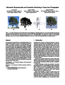
Fig. 1. Illustration of the spatial arrangement used for forward and backward projection. The scene combines volume regions for the attenuation µ-map and the estimated activity.

Function (BSDF) as used in Eq. 1. It essentially describes the probability distribution for different outgoing directions for a given incoming direction of a photon of given energy. Computationally we perform a Monte-Carlo simulation of the photon paths. Our current implementation works for ML-EM and SART. The sampling and integration of the volumetric scene is governed by a number of well defined parameters that can be controlled by the user (e.g., number of sampling rays per camera pixel, jittered or regular). It is possible to reconstruct volumes of different resolution, independent of the resolution of the given projections. Thus, a multi-resolution approach can be incorporated, starting at a coarse resolution for the reconstruction volume and then using finer sampling in subsequent iterations. V. D IFFERENT ATTENUATION CORRECTION SCHEMES IN

distribution. It is implemented as a 3-dimensional camera that samples the incoming flux at discrete volume locations. In the forward projection the volume becomes a three-dimensional radiating volume that is emitting photons with a distribution of the current activity estimate f (k) . The participating medium can be set up to have a certain density distribution and additional scattering, absorption, and emission properties. The

THE BACK PROJECTION

Using our framework as a test environment for different algorithmic configurations we are particularly interested in the effects of different attenuation correction schemes in the back projection of ML-EM and SART. As already mentioned in the explanation on Eq. 7 we may used different projection operators (i.e. systems matrices) in the forward and backward projection. While attenuation correction in the forward projection step is well defined it is not quite clear which scheme for the back projection provides optimal convergence behaviour. Therefore we implemented different methods and applied them to the two different reconstruction algorithms. When tracing a ray back into the volume we can perform attenuation weighting in different ways, as depicted in Fig. 3. The different forms of attenuation correction shown there can Illustration of different attenuation schemes 4.5

4

µ-map

Fig. 2. The activity distribution is reconstructed at the intersection of the projective light sources. These illuminate the volume with an intensity pattern (e.g. a correction images). For illustration purposes this projection is caught by a plane at the bottom of the scene.

attenuation

3.5

inverse atten. 3

inverse

2.5

light sources surrounding the volume (see Fig. 2) use the structural information from the experimental projections or, later in the process, calculated correction projections to update the reconstructed volume. We use the same geometrical scene setup for forward and backward projection (ML-EM approach) or select a subset of the projections (OS-EM). We use several light sources (one for each projection) simultaneously to cast the correction projections onto the volume. As mentioned above, the difference between forward and backward projection is in the direction in which the light is propagated. Essentially, we are inverting the path of the photons, which - according to the Helmholtz reciprocity principle - is physically plausible. After the scene is set up for the forward projection, it is the choice of a volumetric integration method that will decide about the complexity of the effects that are being modeled. In our current setup only direct photon paths are considered. To model first and higher order scattering an additional preprocessing step of volumetric photon mapping has to be performed. We are experimenting with photon tracing in both forward and backward directions. It is possible to follow photons through the volume considering different scattering properties. These are captured by the phase function p. This function p is also known as Bi-directional Scatter Distribution

µ-scale

2

1.5

uniform

1

normal

0.5

0

0

20

40

60

80

100

120

140

160

180

200

distance along the ray

Fig. 3. Different attenuation correction schemes to be used in the back projection step. The dashed line indicates the underlying µ-map. The effect of the parameter µ-scale is to multiplicatively weight the attenuation.

be implemented through a scaling α, weighting the µ-map bi↔j = e−α

Rt 0

µ(p+sω,ω)ds

.

(8)

This coefficient α is also referred to as µ-scale in the following text. Performing forward, uniform, or inverse attenuation correction can be implemented by choosing α to be 1, 0, or −1, respectively. For α = 1, bij = aij . This is the setup we have used in our evaluation as discussed in the following section. A discretized form of Eq. 8 is derived in appendix A.

70

VI. R ESULTS FOR I TERATIVE RECONSTRUCTION METHODS For our tests we are using the MCAT phantom [15] with a resolution of the projections of 128 × 128. Our software runs on a computer with 2.2 GHz AMD Athlon CPU. The timing of the forward projection is independent of the resolution of the reconstructed volume, because ray tracing is an imageorder algorithm. This means that its runtime linearly scales with the effort spent on sampling the scene. It is influenced by the number of pixels in the projection and the number of rays cast per pixel. A forward projection step takes about 89s for all 64 projections for a low-discrepancy sampling with 8 rays per pixel [12]. Other timings are 44.8s and 16s with four and one ray per pixel, respectively. A full backward projection of all 64 correction images on a 1283 volume takes 292s. For a 643 volume this reduces to 38.6s and on 323 it just takes 4.3s. This emphasizes that tremendous speedup can be gained from a multi-resolution reconstruction. We have run the iterative reconstruction for both methods, SART and ML-EM employing different settings for the attenuation in the back projection step as mentioned in section V. The results of this experiment are shown in Fig. 4. The RMSE

Different schemes of attenuation correction in the back projection

6.5

6

5.5

5

4.5

4

3.5 µscale=1 µscale=0 µscale=-0.2 µscale=-0.3 µscale=-0.4 µscale=-0.45 µscale=-0.55 MLEM no AC

3

2.5

2

1.5

2

4

6

8

10

12

14

# iterations

Fig. 4.

Convergence when using different attenuation correction schemes.

shown curves indicate convergence behaviour of the algorithm under different configurations. The root √ mean squared error is calculated at RM SE = kf (k) − f k/ J, where J is the number of elements in f or # of voxels and k·k denotes the 2-norm. The key point in this graph is that uniform attenuation correction (using µ-scale=0) outperforms forward attenuation correction. This is the case for both ML-EM and SART. Furthermore, inverse attenuation correction (µ-scale< 0) potentially improves convergence of SART. This can only be observed up to a certain level. The one divergent curve for µ-scale= −.55 indicates the amount of inverse attenuation where the method becomes instable. While we do not consider this a final result with respect to attenuation correction, we do see this as an interesting pointer for further investigation. The reconstructions after the few iterations of our renderingbased SART implementation are shown in Fig. 5. The framework allows for flexible adjustment of different reconstruction algorithms and their inherent parameters. Attenuation and scatter can be incorporated into the system, by adjusting the absorption and scatter properties of the medium. In particular, the phase function will allow for an effective implementation of the Klein-Nishina formula for Compton scatter.

60 50 40 30 20 10 0

Fig. 5. Effect of inverse attenuation correction in SART (middle, µscale=−.45) compared to no-AC (left) and the truth volume (right).

VII. GPU- BASED ACCELERATION OF M EDICAL R ECONSTRUCTION Recent developments in programmable graphics processing units (GPUs) have made them capable of general purpose computation [18], so they are no longer limited to traditional graphics rendering tasks for which they were originally designed. GPUs can be modeled as a streaming architecture; a massively parallel computational model where each screen pixel is a (limited) processor. For medical image reconstruction, previous research in using GPUs for acceleration ([3], [21]) has shown speed increases of over an order of magnitude compared to pure software implementations. This is significant because iterative methods which may have once been too computationally expensive are now fast enough to become practical for clinical use. One important feature of current generation graphics hardware is the fragment shader which allows for a wide range of calculations to be done in a highly parallelized manner. Floating point precision has also been recently introduced in commodity graphics hardware which allows GPUs to manipulate 16 and 32-bit numbers per color channel instead of only 8-bit numbers. Details can be found in [19], [17], and [20]. Our GPU accelerated EM reconstruction implementation extends Chidlow and M¨oller’s work [3] and modernizes it to make better use of current graphics hardware. GPUs that were available at the time of their research were limited to 8-bits of precision per colour component. They devised a careful bitsplitting strategy where the 16- bit input data was split into four pieces before it was transferred to the graphics card. After rendering, they read back the values and recombined them into main memory using the CPU to achieve 16- bits of fixed point precision. The volume being reconstructed was stored in main memory using floats and stored on the graphics card in texture memory as 8-bit channels using their bit-splitting approach. They could account for values greater than 255, but lost the fractional part of the number since each value was rounded to the nearest integer. Our implementation uses the floating point precision pipeline. Forward projection and back projection is accomplished similarly to [3], with some exceptions. The bit-splitting and recombining of values using the CPU is no longer needed. Instead of reading values from the framebuffer and accumulating values in main memory, we render to an off-screen floating point pixel framebuffer with blending enabled. In the EM correction step, since we no longer have to encode values as bytes, we’re able to have correction values greater than 2.0. Chidlow’s implementation had to clamp correction values to the range [0..2] and encoded them as [0..255], with 1.0 corresponding to 127. The clamping limited the algorithm’s potential, by only allowing an increase in a voxel’s intensity by a factor of two at each step. However, without this restriction, the increased convergence rate is only noticeable for a small number of iterations. As noted in [3], the number of iterations required to correct for their range

clamping is an order of magnitude less than the number of iterations run in a typical reconstruction (upwards of 80 for EM). In practice, OSEM may gain more from the removal of the clamping since a small number of iterations is typical. Quality is comparable to a pure software implementation. Performance is 1.3× faster than the previous GPU implementation (see table I), whereas the previous GPU implementation is 9.4× faster than a pure software implementation. Results were obtained on an AMD Athlon 2000 CPU and a GeForce6 6600GT GPU.

where J is the number of points in the grid. The actual number of points iterated over in the implementation is much smaller because of the limited support of kernel h. The same method of interpolation is now used to determine the contribution of the throughput of all ray points xs1..M to a grid point xj , which gives us the final throughput between grid point j and projection pixel i: bi↔j =

M X

m=1

EM EM EM EM

no AC no AC with AC with AC

Time (sec) 45.0 34.5 67.5 47.2

Chidlow Float Chidlow Float

Avg iteration (sec) 1.1 0.86 1.7 1.2

bi↔xsm h(xsm − xj ).

(12)

Here and in the previous equations we have neglected the fact that the discretization of the integral only supplies us with an approximate value for the actual throughput. The one given here is ’actual’ in the sense of what is implicit in the implementation. The elements aij can be seen a special case of bij with α = 1.

TABLE I C OMPARISON BETWEEN C HIDLOW ’ S AND FLOATING POINT RECONSTRUCTIONS FOR 40 EM ITERATIONS .

R EFERENCES

VIII. S UMMARY We are pursuing two different goals with this research. On the one hand the presented framework gives us a flexible and scriptable environment allowing the testing of novel algorithms (e.g. different system matrix configurations, multi-resolution approaches, etc.). Secondly, by building a bridge to common computer graphics algorithms we are able to speed up the underlying reconstruction by taking advantage of the vast body of research on real-time rendering improvements from GPU accelerated algorithms as mentioned above. Two main directions for future work are the use of photon mapping for scatter correction and reconstruction on an optimal grid structure. IX. A PPENDIX A: S YSTEMS MATRIX ELEMENTS The effect that radiation fj at a grid location xj has on a detected value gi at position xgi is determined by accumulating the throughput bi↔xsl of each of the points xsl = xgi + l∆sω sampled at distance ∆s along a ray of direction ω, orthogonal to the projection screen. The i ↔ j indexing is equivalent to ij, but emphasizing the fact that this weighting is independent of whether photons are traveling from detector to volume location of vice versa. More details of be shown as we work towards the result in Eq. 12. The derivations presented here are based on Chidlow’s thesis [2]. First, we need to be able to determine the throughput of a single sample position xsl , which is governed by the attenuation properties at the positions 1..L up to the one under consideration. Each of them can be computed by discretizing Eq. 8 as follows bi↔xsl = e−α∆s

PL

l=1

µ(xsl )

.

(9)

Its equivalent recursive form bi↔xsl+1 = bi↔xsl e−α∆sσt µ(xsl )

(10)

is what makes implementation practicable. The distribution of the attenuation, the µ-map, is given on a discrete grid as µj at grid point locations xj . It can be interpolated at a sample point position xsl using a reconstruction kernel h: µ(xsl ) =

J X j=1

µj h(xsl − xj ),

(11)

[1] Freek J Beekman, Hugo W A M de Jong, and Eddy T P Slijpen. Efficient spect scatter calculation in non-uniform media using correlated monte carlo simulation. Phys. Med. Biol., 44:N183–N192, 1999. [2] Ken Chidlow. Graphics hardware accelerated iterative reconstruction for SPECT imaging. Master’s thesis, Simon Fraser University, 2003. [3] Ken Chidlow and Torsten M¨oller. Rapid emission tomography reconstruction. In Workshop on Volume Graphics 2003 (VG03), Tokyo, July 2003. [4] Gabor T. Herman. Image reconstruction from projections: the fundamentals of computerized tomography. Academic Press, San Francisco, 1980. [5] H. Malcolm Hudson and Richard S. Larkin. Accelerated image reconstruction using ordered subsets of projection data. IEEE Trans. on Med. Imag., 13(4):601–609, December 1994. [6] H. W. Jensen and P. H. Christensen. Efficient simulation of light transport in scenes with participating media using photon maps. In Proc. of SIGGraph 25th Conf. on Comp. Graph., pages 311–320. ACM Press, 1998. [7] Henrik Wann Jensen. Realistic Image Synthesis Using Photon Mapping. AK Peters, July 2001. [8] James T. Kajiya and Brian P. von Herzen. Ray tracing volume densities. Computer Graphics, 18:165–174, July 1984. [9] Arie E. Kaufman, editor. The Application of Transport Theory to Visualization of 3D Scalar Data Fields, 1990. [10] J. Kniss, S. Premoze, Ch. Hansen, P. Shirley, and A. McPherson. A model for volume lighting and modeling. IEEE Trans. on Visualization and Computer Graphics, 9(2):150–162, April-June 2003. [11] Nelson Max. Optical models for direct volume rendering. IEEE Trans. on Vis. and Graph., 1(2), 1995. [12] Matt Pharr and Greg Humphreys. Physically Based Rendering from Theory to Implementation. Morgan Kaufmann, 2004. [13] L. A. Shepp and Y. Vardi. Maximum likelihood reconstruction in positron emission tomography. IEEE Trans. Medical Imaging, 1(2):113– 122, 1982. [14] Peter Shirley and R. Keith Morley. Realistic Ray Tracing. A K Peters, 2003. [15] B. Tsui, X. Zhao, G. Gregoriou, D. Lalush, E. Frey, R. Johnston, and W. McCartney. Quantitative cardiac SPECT reconstruction with reduced image degradation due to patient anatomy. IEEE Trans. on Nucl. Science, 41:2838–2844, 1994. [16] R.G. Wells, A. Celler, and R. Harrop. Analytical calculation of photon distributions in SPECT projections. IEEE Trans. on Nuclear Science, 45:3202–3214, December 1998. [17] Joint work. Ati: Developer, the inside track. In http://www.ati.com/developer/, 2005. [18] Joint work. General-purpose computation on GPUs. In http://www.gpgpu.org, 2005. [19] Joint work. Nvidia: The source for gpu programming. In http://developer.nvidia.com/, 2005. [20] Joint work. Opengl 2.0 specification. In http://www.opengl.org/, 2005. [21] Fang Xu and Klaus Mueller. Towards a unified framework for rapid computed tomography on commodity gpus. In IEEE Medical Imaging Conference (MIC) 2003, Portland, October 2003. [22] Fang Xu and Klaus Mueller. Accelerating popular tomographic reconstruction algorithms on commodity PC graphics hardware. IEEE Transaction of Nuclear Science, pages ???–???, 2005. (to appear).