Though Wireless Sensor Network (WSN) research activi- ties are going on for ..... to wireless sensor networks can yield multiple benefits: ⢠With regard to the ...
Using Transaction Level Modeling Techniques for Wireless Sensor Network Simulation Markus Damm, Javier Moreno, Jan Haase, and Christoph Grimm Institute of Computer Technology Vienna University of Technology, Austria {damm|moreno|haase|grimm}@ict.tuwien.ac.at
Abstract
cable harness within the car, which is already very high with cable lengths up to 2 km, the use of wireless communication becomes imperative. The automotive application scenario will usually have a central unit (CU), which collects and processes the various sensor data. The sensors in use are heterogeneous regarding duty cycle, power consumption, operation distance (also with respect to radio frequency (RF) barriers), and power supply. Part of the RF sensor nodes might be attached to the car’s electrical power system, thus are provided with a virtually infinite power supply. While most of the nodes might be only designed to transmit data, some nodes will be also able to receive and forward messages within a multi-hop network. Certain sensor nodes will also be attached to the car’s bus system, such that we actually face a mixed wireless / wired sensor network (see Figure 1).
Wireless Sensor Networks are gaining more and more importance in various application fields. Often, energy autonomy on the node level is an essential nonfunctional constraint to be met. Therefore, when simulating such networks, the energy consumption on the node level has to be included into the simulation. To make this time consuming task feasible, an overall simulation speedup on the network level is desirable. In this paper, we propose to use techniques similar to those used in Transaction Level Models of Bus Systems. 1
1
Introduction
CU
Though Wireless Sensor Network (WSN) research activities are going on for several years, there is still an energy autonomy gap between application requirements on one side and the WSN-node and -platform abilities on the other side. Since the power consumption of a node is influenced also by network level aspects like the protocol used, it is important to include the network level down to the node level when using simulation as a tool within the design process. This work is done within the Project SNOPS (Sensor Network Optimization by Power Simulation), which targets wireless sensor networks (WSN) in general. However, a special emphasis lies on wireless sensor networks in the automotive sector. An obvious application here is a Tire Pressure Monitoring System (TPMS), which is commonly used today.It is projected that the use of wireless sensors in the automotive sector will become increasingly ubiquitous in the future, especially for convenience purposes (e.g. environmental sensors). To control complexity and size of the
Bus-connection
Figure 1. A mixed wireless/wired automotive sensor network Apart from the application scenario, SNOPS also investigates a specific energy optimization strategy by accompanying the sensor node’s microprocessor by custom coarsegrain reconfigurable hardware blocks, which relieve it from simple, yet power-intensive tasks (see [4] and [3] for details). To sufficiently assess the power savings achieved by this method, the simulation of the microprocessor has to include an ISS. Within an overall network simulation, this ap-
1 This
work is conducted as part of the Sensor Network Optimization by Power Simulation (SNOPS) project which is funded by the Austrian government via FIT-IT (grant number 815069/13511) within the European ITEA2 project GEODES (grant number 07013).
1
978-3-9810801-6-2/DATE10 © 2010 EDAA
RF-connection
proach can turn out to be very expensive with respect to simulation performance. To make up for this costly detailed node level simulation, a lightweight network level simulation approach is needed. We propose to use techniques similar to Transaction Level Modeling (TLM, see [1, 7]), a modeling and simulation paradigm for bus-based systems, to get such an approach. The remainder of this paper is organized as follows: In Section 2, we review some of the related work, including the PAWiS project, which is a predecessor to the SNOPS project. Also, we give a short introduction to TLM in Subsection 2.2. In Section 3, we discuss how to translate the concepts of TLM to WSN simulation, and show in Section 4 how this can be achieved using the current TLM 2.0 mechanisms. In Section 5, first results are presented, before concluding in Section 6.
2
the Air. The Air model includes calculating signal power received, the bit error ratio and modeling collisions. As it is in OMNeT++, every communication between modules is done through messages. The PAWiS framework implements its own messages, inheriting from the OMNeT++ basic message class. Each communication layer can define their own message kind, with the required fields, and encapsulate messages received from the upper layer.
2.2
TLM is mainly intended for modeling and simulation of systems using busses for communication. The main idea is to abstract the low-level events occurring in bus communication (“pin wiggling”) into a single element called transaction. That is, the communication is abstracted in a way that focuses on data transfers between system parts, possibly together with more or less accurate timing estimates for the transfers. TLM is a technique mainly employed in C-based design, and especially within SystemC [8]. With TLM 2.0 [1], there exists an OSCI standard with a focus on model interoperability with standardized transaction objects and abstract protocol phases. The standard transaction class in TLM 2.0 is called generic payload, and has attributes like a command (read or write), a target address and a data section, which basically sets a focus on memory mapped busses. Transactions are passed by reference via method calls among the different components of the system model. For example, a read request from a CPU to a Memory module together with the resulting data transfer can be captured by one transaction. In TLM 2.0, every component in the system model basically assumes one of three roles:
Related work
In [10] SystemC AMS was used to simulate nodes of a WSN at architecture level, including analog components. In [2] SystemC was successfully used to co-simulate the hardware and software parts of a wireless sensor network. Some preliminary tests were made with a pure SystemC model with excellent results. However, the lack of support for modeling upper layer network communication in SystemC finally led to the usage of NS-2 [6] to model the network. In [12], a protocol for cooperative MIMO mobile sensor networks was proposed. For the modeling, TLM and SystemC was used, resulting in a very fast and efficient simulator that permitted to evaluate the network performance. However, no details were given on how TLM was used exactly.
2.1
Transaction Level Modeling
• Initiators (e.g. CPU models) create new transactions.
The PAWiS framework
• Interconnects (e.g. busses and routers) do forward and possibly modify transactions.
During the PAWiS (Power Aware Wireless Sensors) project [5], a simulation framework for wireless sensor networks was developed. It is based on the OMNeT++ Discrete Event Simulation System [9]. The PAWiS framework models the internal structure of sensor nodes and the communication among them. Each node is built as a virtual prototype divided into functional blocks, which are mapped into modules. The PAWiS Framework provides the module interfaces, as well as the messages used to communicate between them. Due to the dedicated focus on power optimization, the framework provides a Power Meter where reporters, associated to modules, log the power consumption values. In addition to modules and the message infrastructure, which are an extension of those provided by OMNeT++, the PAWiS framework provides also a model of the environment, called
• Targets (e.g. memories and I/O components) are the final destinations of the transactions. The lifetime of a transaction can have various granularities. If it is a single time span (which might be zero), this is usually modeled using the so called loosely timed coding style. This coding also has the additional feature that temporal decoupling can be used, which means that initiators can run ahead of the global simulation time by maintaining a local timing offset, and synchronize with the global simulation time either periodically or depending on certain circumstances. This technique allows for a further simulation speedup, since it reduces context switches. It is also possible to subdivide the lifetime of a transaction into different phases (accompanied by respective 2
method calls), e.g. capturing address phase, data phase and latencies. This is known as the approximately timed coding style. The TLM 2.0 standard foresees several method interfaces for passing transactions, with the most important ones being the blocking and the nonblocking interface. The blocking interface has just one method implemented by targets, namely b transport(transaction, time-offset), and is usually chosen when using the loosely timed coding style. The name ”blocking” results from the fact that an implementation of this method is allowed to call a SystemC wait(time/event). The time offset parameter passed with the transaction indicates when the transaction is valid with respect to the current simulation time. The nonblocking interface, which is used for the approximately timed coding style, has two similar methods, one for the initiator side and one for the target side, with an additional phase parameter. For details, consult [1].
3
Master1
SN1
Master2
SN2
pin wiggling, signals
Environment
Bus
Slave1
Slave2
SN3
Abstraction
SoC Initiator1
modulated waves, signals
WSN SN1
Initiator2
SN4
SN2
transactions, method calls
TLM-Interconnect
Environment model data packets, method calls
Target1
Target2
SN3
SN4
TLM and WSN Figure 2. Similar abstractions for SoCs and WSNs (SN: Sensor Node)
At first glance, the TLM 2.0 approach seems not to be very useful regarding wireless sensor network simulation at the network level, where no dedicated busses, routers or arbiters are used. But from a simulation point of view, an environment model (e.g. as it is implemented in the PAWiS framework [11]) behaves not much different from a bus model in TLM 2.0 (see Figure 2): it gets transmitted data packets (which correspond to transactions), and forwards them. However, it is important to note the differences:
the packet from the node, has to determine all nodes which are able to receive the packet, and forward the packet to them (See Section 2.1). A node then decides by itself if it receives this packet completely: If the packet contains a target ID, it might stop receiving upon decoding a target ID not matching its own ID (the same holds if message IDs similar to the operation of a CAN bus are used). Note that it is important to model these canceled receiving attempts, since they influence the power consumption in the network. For simple functional verification, it could make sense to not model these effects. That is, the environment could be modeled such that it only forwards the data packet to the node with the matching target address. But even in this case, forks can occur: if a node routes a packet, it might route it to more than one node, depending on the routing strategy used. Also, broadcast messages might be used which have to be distributed through the whole (or a part of the) network, e.g. to exchange routing information. In contrast to this, a transaction in a TLM model is always passed along a straight path (see Figure 3), where the accesses to the transaction are non-concurrent. In turn, if we choose to represent the transmission of a data packet through a WSN by a single transaction object, we might have concurrent accesses to it. Obviously, the TLM approach has to be altered to be useful for wireless sensor network simulation. Fortunately, the TLM 2.0 standard is very flexible. It is possible to extend the generic payload by additional attributes (e.g sig-
• A TLM bus model will be part of a later implementation, while the environment model is an estimate of the operating conditions the implementation will face. • In WSNs, no memory map is used, therefore using READ and WRITE commands also makes no sense. • The smallest information unit in the TLM standard is a byte, whereas in WSNs, the data granularity refers to bits. • A WSN node might be the source as well as the destination of data packets, while it might also be used to route data packets. Therefore, from the TLM point of view, it acts as initiator, target and interconnect. • While a transaction in a usual TLM model is passed along a straight path through the system, the transmission of a data packet in a WSN network might fork. The last point requires some explanation. In a WSN, a data packet transmitted by one node can be received by all nodes close enough. Therefore the environment model, which gets 3
whole system’s (or certain critical node’s) power consumption, and use this information to optimize WSN protocols and routing strategies.
Initiator2
Target1 Target2
Component involved in transaction
Target3
Interconnect2
Initiator1
Interconnect1
TLM-model
Target4
4
Target5
Since the transaction is a pivotal concept in TLM 2.0, it is vital to find a suitable adaption to WSN modeling. While some of generic payload attributes of TLM 2.0 are not suitable for our purposes (e.g. byte enable or streaming width), we have to add others (e.g. signal strength, transmission duration). Fortunately, with the generic payload extension mechanism there is an appropriate tool available for this purpose. Informally, a generic payload extensions can be thought of as a ”Post-it” attached to the generic payload. Technically, it is an arbitrary C++ structure implementing the TLM 2.0 generic payload extension interface (see [1]). It is possible to attach arbitraryly many extensions of different types (but only one of each type) to a generic payload. Our adoption of the TLM approach to WSNs works as follows: When a node transmits a data packet, it generates a new generic payload, with the data going into its data section and the ID of the final target node going into the address parameter. It then attaches a extension with additional information, e.g. to which node to route to, or the signal strength, and sends the transaction to the environment model. The environment model now determines which nodes are able to receive the data packet associated to the transaction, and sends the transaction to them. Keeping the transaction level point of view is the most demanding part of this implementation. In a message implementation, like the one in PAWiS, each node owned a message and they were duplicated when sending to several nodes. However, in the transaction approach, a single transaction must cover the whole communication process. As the transaction is likely used by several nodes at the same time, data modifications in the transaction may lead to inconsistencies. Also, some of the data is different for every node, e.g. the signal strength. Therefore, we use a second extension for the transactions send from environment to the nodes. We refer to this extension as node extension, while the other is called environment extension. The basic data contained in the node extension is the same, but now organized using the map data structure from the C++ standard template library, where the key is the ID of the node the transaction is sent to. Since a transaction might pass a node more than once, we keep the data within a dynamic array, and keep a map of indexes (again with the node ID as a key) to indicate to the respective node which array entry holds the actual data. However, each node can in principle also access data not intended for it. Therefore, transaction data must be interfaced so that only permitted operations can be carried out and the integrity of the trans-
Component not involved in transaction
WSN-model SN4
SN1
SN7 SN9
SN3
SN6
SN2 SN8
SN5 SN10 Node involved in routing
SN11 Node not involved in routing
Implementation
Node receiving, but not involved in routing
Figure 3. TLM Transaction path versus a WSN packet path
nal strength or bit error rate for the case at hand), but the TLM 2.0 interfaces can also be used with an entirely custom transaction class. Also, an extended or entirely custom set of phases can be introduced, which could be used to capture typical wireless communication steps like carrier sensing. A successful adaptation of the TLM 2.0 approach to wireless sensor networks can yield multiple benefits: • With regard to the mixed wireless / wired sensor network scenario, we stay within a modeling paradigm where bus modeling is straightforward. This is an issue not addressed by the PAWiS framework properly. • We can benefit from the general simulation performance enhancement prospects of TLM. • If TLM is also used to model the sensor nodes internals, it might be possible to achieve seamless integration of node and network simulation. Moreover, by associating power consumption information to transactions, we can get a whole new view on power consumption in a wireless sensor network by introducing concepts like the power consumption of a transaction. We can determine in how far certain transactions influence the 4
Section 2.1, which uses the ordinary message perspective and is based on the OMNeT++ simulation environment.
action is preserved. SN1
1
2
Environment
SN3
3
Environment
2
4
SN5
4
SN2
Measure Temperature (t) (periodic)
SN4
1
2
3
4
GP
GP
GP
GP
target data
5 1.5
target data
5 1.5
target data
5 1.5
target data
ENV-EXT
ENV-EXT
ENV-EXT
ENV-EXT
route-adr 3 strength 7.5
route-adr 3 strength 7.5
route-adr 5 strength 6.3
route-adr 5 strength 6.3
NODE-EXT
2
route-adr 3 strength 0.9
3
route-adr 3 strength 0.3
NODE-EXT
|Δt|>1°C
5 1.5
yes Send Message
NODE-EXT
2
route-adr 3 strength 0.9
2
route-adr 3 strength 0.9
3
route-adr 3 strength 0.3
3
route-adr 3 strength 0.3
4
route-adr 5 strength 0.7
5
route-adr 5 strength 1.1
listening? no yes
Sink node? yes
Listen
Figure 4. A generic payload with WSN extensions in the course of a packet transmission
Receive Message
Discard Message
no no
TTL>=0 yes Forward Message
Figure 5. Flowchart of node operation in the network simulated. On the left, message generation of ordinary nodes. On the right, tasks carried out whenever a message arrives.
Figure 4 shows an example (without vectors). As the transaction is sent to the environment the first time in step 1, it only contains the environment extension. Before the environment passes it to nodes 2 and 3 in step 2, it adds the node extension with entries for these two nodes. Note that the environment extension is still present, but is not accessed by the nodes. In step 3, node 3 reuses the environment extension before it passes the transaction to the environment, which then adds information for node 4 and 5 in step 4. The additional benefit of this approach that we get a complete history of the data transfer associated to the transaction. Since the correlation of all single transmission and receiving events caused by this data transfer is kept, we can use this information to e.g optimize routing strategies with respect to power consumption, if we add the consumed power by each node to the node extension. It is also conceivable to add an additional extension for power consumption or other kinds of ”simulation meta-data” and, regarding the network architecture, to add extensions for each network layer. In general, adding any kind of user defined extension depending on the protocols used is possible.
5
no
Message Received
The example provides an application and a basic MAC layer to determine when the node is listening and messages can be received. In addition, to be able to test how multi-hop communication performs, a very simple routing layer has been implemented. The example network consists on a sink node, which is listening all the time and does not generate messages, and ordinary nodes, which generate messages and are able to listen during restricted periods of time. The application implemented consists of nodes measuring temperature periodically. Two flowcharts, one for each possible event, periodic sensing or message reception, are shown in Figure 5. If the difference between the temperature measured and the last sent value is significant, the new value is sent through the network. The destination of temperature data is always the sink node. However, it may not be directly reachable. Therefore, ordinary nodes must work also as transition nodes. Every node in the network which is listening and within the range of the sender node, receives the message and checks errors and integrity. If the receiver is not the sink node, it forwards the message. To avoid infinite loops, a Time-To-Live value is attached to the message, which decreases on every hop. If this value reaches 0, the message is discarded. Error calculation must be implemented out of the framework too, as it depends on modulation. In the example, errors are calculated for a 4-QAM modulation.
Results
In this section a simple example of wireless network is presented and implemented with our framework, using the transaction level point of view described in Section 4, and with SystemC as the simulation kernel. A similar example is implemented using the PAWiS Framework, described in 5
Simulation results, shown in Table 1, are intended to check the new TLM-based framework performance, in terms of simulation speed. This results are compared with those obtained using the PAWiS framework.
Considering the results, this new perspective promises also a significant improvement in simulation performance.
Table 1. Simulation Time Results PAWiS SNOPS Nodes: 3 2,462s 2,397s Time: 24h Nodes: 15 47,783s 32,819s Time: 24h Nodes: 25 3m 1m 32,27s Time: 24h 3,6s
[1] J. Aynsley. OSCI TLM-2.0 Language Reference Manual. Technical report, Open SystemC Initiative, 2009. [2] F. Fummi, D. Quaglia, F. Ricciato, and M. Turolla. Modeling and simulation of mobile gateways interacting with wireless sensor networks. In DATE ’06: Proceedings of the conference on Design, automation and test in Europe, pages 106–111, 3001 Leuven, Belgium, Belgium, 2006. European Design and Automation Association. [3] J. Glaser, J. Haase, M. Damm, and C. Grimm. Investigating power-reduction for a reconfigurable sensor interface. In Proceedings of the Austrian National Conference on the Design of Integrated Circuits and Systems (Austrochip 2009), Graz, Austria, 7. 2009. [4] J. Haase, M. Damm, J. Glaser, J. Moreno, and C. Grimm. Systemc-based power simulation of wireless sensor networks. In Proceedings of the Forum of Design Languages, 2009. [5] S. Mahlknecht, J. Glaser, and T. Herndl. PAWiS: Towards a Power Aware System Architecture for a SoC/SiP Wireless Sensor and Actor Node Implementation. In Proceedings of 6th IFAC International Conference on Fieldbus Systems and their Applications, pages 129 – 134, Puebla, Mexiko, 14.15. Nov. 2005. [6] S. McCanne and S. Floyd. NS Network Simulator - version 2. Website, 1996. http://www.isi.edu/nsnam/ns. [7] Open SystemC Initiative. OSCI TLM2.0. http://www.systemc.org. [8] Open SystemC Initiative. SystemCTM . http://www.systemc.org. [9] A. Varga. The OMNeT++ discrete event simulation system. In European Simulation Multiconference (ESM’2001), Prague, Czech Republic, 2001. [10] M. Vasilevski, F. Pecheux, N. Beilleau, H. Aboushady, and K. Einwich. Modeling and refining heterogeneous systems with systemc-ams: Application to WSN. Design, Automation and Test in Europe Conference and Exhibition, 0:134– 139, 2008. [11] D. Weber, J. Glaser, and S. Mahlknecht. Discrete Event Simulation Framework for Power Aware Wireless Sensor Networks. In Proceedings of the 5th International Conference on Industrial Informatics, INDIN 2007, volume 1, pages 335–340, Vienna, Austria, 23-26 July 2007. [12] Q. Zhang, W. Cho, G. E. Sobelman, L. Yang, and R. Voyles. Ubiquitous Intelligence and Computing, pages 508–516. Springer Berlin/Heidelberg, 2006. ISBN 978-3-540-380917.
References
Results for 24 hours of simulated time and different amount of nodes are presented. In the first simulation the number of nodes is 3, which is not demanding at all, so both frameworks require very little time. The SNOPS framework required 2,6% less time, which is almost negligible. In the second simulation, a network with 15 nodes is tested. In this case, the SNOPS framework improved PAWiS results by 31,32%, which makes a significant difference. With 25 nodes the improvement is even higher, with 49,7% less time for the SNOPS framework.
6
Conclusion and Outlook
In this paper, a new TLM-inspired approach for Wireless Sensor Network simulation was presented. The prospects of using TLM within a WSN simulation framework is twofold. Apart from yielding a fast simulation framework with new capabilities, it is also a way to explore in how far the TLM paradigm has to be altered to be useful for the area of WSN modeling and simulation. Currently, some aspects of the TLM 2.0 mechanisms (mainly within the generic payload) are ”misused” in the sense that we depart from the original semantics, while other aspects are neglected because they are of no apparent use. Since this is done within a single framework, which does not need to be TLM 2.0 compliant, this poses no problem, especially considering that the end user does not have to deal with these aspects of the framework directly. Note however, that with respect to timing (i.e. considering the loosely and approximately timed coding styles), the altered network level TLM should work well together with possible TLM 2.0 models on the node level. However, the experience gained could show the way for an approach for general wireless network modeling and simulation which might play a similar role like the TLM 2.0 approach for bus oriented modeling and simulation. That is, an approach for SystemC based modeling by providing a standardized extension library for model interoperability in wireless networks. 6