E.V. Ivanovich, K. Hamid Journal Water Sustainability 2 (2014) 75-87 Journal of Water Sustainability, Volume/ 4, Issue 2,ofJune 2014, 77-89
1
© University of Technology Sydney & Xi’an University of Architecture and Technology
Using Turbidity to Determine Total Suspend Solids - Field Measurement: Dez Dam Reservoir Elfimov Valery Ivanovich, Khakzad Hamid* Division of Civil Engineering, Peoples’ Friendship University of Russia, Moscow 117198, Russia
ABSTRACT One part of water quality, Total Suspended Solids (TSS), is a reliable indicator of other pollutants, particularly nutrients and metals that carried on the surfaces of sediment in suspension. The measurement of TSS (APHA, 1995) is time consuming, and much research has been done to correlate secondary parameters to TSS, but the process of turbidity measurement is simpler and faster than the process of TSS measurement. The correlation between TSS and turbidity established to provide more efficiency in predicting total suspended solids concentration in dam reservoir. A positive correlation between total suspended solids concentration and turbidity level, suggested measurement of turbidity possibly, is the most profitable option for estimating total suspended solids concentration in dam reservoir. A random study was conducted from Jan 2002 to July 2003 in Dez dam reservoir. Dez dam reservoir in Iran is facing a serious sedimentation problem and its dead volume will be quite full in the coming 10 years, and now the inflow water in hydropower conduit system is becoming turbid. These results strongly suggest that, turbidity is an appropriate monitoring parameter where TSS must be evaluated and the measurement of turbidity levels has the potential to replace the measurement of TSS concentrations. Keywords: Dez Dam Reservoir; total suspended solids; turbidity; water quality
1.
INTRODUCTION
The turbidity unites reported in Nephelometric Turbidity Units (NTU), which is a measurement of the intensity of light being scattered when light is transmitted through a water sample. Turbidity is affected by more than just particle concentration. Water color due to dissolved solids (Malcolm, 1985) and temperature, as well as the shape, size and mineral composition of particles (Clifford et al., 1995; Gippel, 1988) can significantly affect a turbidity reading. In addition, comparison of turbidity readings between studies is confounded by a lack of a universal method of turbidity instrumentation.
*Corresponding to:
[email protected] DOI: 10.11912/jws.4.2.77-89
The measurement of TSS (APHA, 1995) is time consuming, and much research has been done to correlate secondary parameters to TSS, such as discharge (Webb and Walling, 1992; Williams, 1989), turbidity (Gippel, 1995; Sidle and Campbell, 1985), and water density (FISP, 1982). Each surrogate has limitations in statistical certainty, predictive power, and logistical coordination. As one of the least expensive and easiest measuring methods, turbidity has been utilized extensively in various environments including streams (Gippel, 1989), lakes (Halfman and Scholz, 1993; Paul et al., 1982), wetlands (Mitsch and Reeder, 1992), and tidal salt marshes (Suk et al., 1998). As a measurement of the attenuation or scattering of a
78
E.V. Ivanovich, K. Hamid / Journal of Water Sustainability 2 (2014) 77-89
light beam by suspended solids (particulate and dissolved) in the water column, turbidity has the potential to provide the most direct measure of particulate concentration.
2. MATERIAL AND METHOD 2.1
Material
This study carried out at the Dez reservoir which is located in south of Iran. The Dez dam (Persian: ) دزis a large hydroelectric dam in Iran, which was completed in 1963 by an Italian consortium. At the time of construction, the Dez dam was Iran’s biggest development project. Dez is 203 m high double curvature arch dam, and the crest of Dez dam is 352 m above sea level. The original reservoir volume was 3315 million m3, and the volume of arrival sediment was estimated at 840 million cubic meters (MCM) for a 50 years period. The minimum and maximum water levels of the reservoir operation are 300 m and 352 m from sea level respectively. Although the project has Table 1
been well-preserved, the project is now more than 40 years old and reaching its midlife period. The useful life of Dez reservoir is threatened by a sediment delta, which is approaching the dam’s intake tunnels. The hydrographic working in 2002 showed that sedimentation reduced useful storage of the reservoir of the Dez dam from 3315.6 MCM to 2700 MCM (19% reduction). Difference between levels of the inlet of turbine and bed surface of deposited sediment is 14 m with the rate of 2 m/year. Therefore, sediment management in the Dez reservoir is essential and of considerable importance. A field measurement program for the measurement of the turbidity current in the Dez reservoir commenced in December, 2002 and finished in June 2003 (Dezab and Acres, 2004). The measurements were taken daily. The program consisted of a series of measurements at various depths and locations across seven cross-sections. The station locations are shown on Fig. 1 and measurements and equipment are shown on Tables 1 to 3.
Measurements at various depths and locations across seven cross-sections
Measurement
Equipment
Depth(from water pressure)
RCM9
Temperature
RCM9
Turbidity
RCM9
Velocity
Vale port current
Suspended sediment sample
Vertical tube sampler
Table 2
Valeport 108 MK II specifications
Property
Type
Range
Resolution
Speed
-
0.03-5 m/s
-
°
Direction
Flux Gate
0-360
0.25°
Temperature
Thermistor
-5-35°C
0.002°C
Electrical conductivity
-
0.1-60 ms/cm
0.001 ms/cm
Pressure
Strain Gauge
100,200,500,1000
0.005% FS
E.V. Ivanovich, K. Hamid / Journal of Water Sustainability 2 (2014) 77-89
Table 3
79
RCM9 specifications
Property
Type
Range
Resolution
Speed
Doppler Current Sensor 3920
0-300 cm/S
0.3 cm/S
Direction
Magnetic compass. Hall effect type
°
0-360
0.35° °
Temperature
Thermistor (Fenwall B32JM19)
-0.64-32.78 C
0.1% of range
Electrical conductivity
Inductive Cell
0-74 ms/cm
0.1% of range
Pressure
Sillicon piezoresistive bridge
0-3500 kPa
0.1% of range
Turbidity
Optical Back-Scatter Sensor
0-1000 NTU
0.1% of flill scale
The first 4 month data gathering was done by Vale port 108 MK II that is capable for measuring current velocity and direction, electrical conductivity, temperature and pressure and calculates salinity, density and speed of sound. Data gathering is direct reading. After the 4th month, a RCM9 instrument was used to collect data. In
Figure 1
addition to the previously mentioned parameters, it can measure water turbidity. Also it is self-recording equipment. Figs. 2 to 5 and Table 4 show a sample of field measurement records on turbidity current in 0.2, 0.6 and 0.8 of maximum depth at A2, B3, C3, E and F stations which were collected in 24 April, 2003.
Measurement Stations
80
E.V. Ivanovich, K. Hamid / Journal of Water Sustainability 2 (2014) 77-89
TSS measurement was done according to American society for testing and materials (ASTM) - D5907 method. TSS range which is measurable by this method is between 4-2000 mg/L. To identify water TSS concentration, water sampling was done in different depths at each station. Water sampling equipment is shown in Fig. 6.
different parameters include current velocity, direction, electrical conductivity, temperature, pH, dimensionless water depth, turbidity and concentration used in this study. The median particle of all samples was less than 0.01 mm, with sediments taken upstream in the reservoir slightly larger than those closer to the dam.
Table 5 shows the ranges and value of Table 4 Sample of field measurement records in 24 April, 2003 Item Date Water level (m) Maximum depth (m) Reservoir inflow(m3/s) Reservoir inflow(m3/s)
Figure 2
Value 24 April, 2003 351 94 590.8 1210.6
Temperature(°C)-Dimensionless water depth (z/H) profiles at A2, B3, C3, E and F
E.V. Ivanovich, K. Hamid / Journal of Water Sustainability 2 (2014) 77-89
Figure 3
Figure 4
81
Current speed (cm/S)-Dimensionless water depth (z/H) profiles at A2, B3, C3, E and F
Current speed (Degree)-Dimensionless water depth (z/H) profiles at A2, B3, C3, E and F
82
Figure 5
E.V. Ivanovich, K. Hamid / Journal of Water Sustainability 2 (2014) 77-89
Turbidity (NTU)- Dimensionless water depth (z/H) profiles atA2, B3, C3, E and F
Figure 6
Water sampling equipment for TSS measurement
E.V. Ivanovich, K. Hamid / Journal of Water Sustainability 2 (2014) 77-89
Table 5
Sample data 15-Mar. -2003 17-Mar. -2003 22-Mar. -2003 23-Mar. -2003 27-Mar. -2003 28-Mar. -2003 29-Mar. -2003 30-Mar. -2003 2-Apr. -2003 6-Apr. -2003 13-Apr. -2003 15-Apr. -2003 16-Apr. -2003 23-Apr. -2003 24-Apr. -2003 25-Apr. -2003
83
Current velocity, direction, electrical conductivity, temperature, pH, dimensionless water depth, turbidity and concentration at A2, B3, C3, E and F stations Sample ID
Dimensionless water depth
EC (mho/cm)
Temp. (°C)
Vel. (cm/s)
Direction (Degree)
Turbidity (NTU)
Conc. (gr/L)
pH
A2
0.91
210.00
13.22
3.52
100.21
34.93
0.28
-
A2
0.93
195.00
13.14
2.05
178.96
18.78
0.15
-
A2
0.94
204.00
13.33
2.05
258.78
17.45
0.10
7.72
A2
0.91
198.00
13.17
4.40
345.97
17.89
0.15
-
A2
0.85
171.00
13.24
57.19
178.61
614.66
6.83
7.88
A2
0.89
132.00
13.05
44.00
172.99
850.00
8.66
-
A2
0.95
126.00
13.30
5.87
174.39
136.40
1.18
-
A2
0.93
126.00
13.00
3.23
167.71
12.73
0.08
-
A2
0.97
108.00
13.52
1.17
93.53
221.55
1.91
-
A2
0.73
174.00
13.26
1.17
287.61
41.14
0.52
-
A2
0.85
159.00
13.24
7.33
260.18
36.45
0.44
-
A2
0.78
204.00
13.40
10.10
136.00
26.00
0.19
-
A2
0.84
183.00
13.46
11.15
40.79
27.06
0.29
-
A2
0.86
-
13.85
97.67
181.43
44.34
0.34
7.89
A2
0.79
-
13.50
37.25
170.88
580.84
5.05
-
A2
0.88
-
13.55
12.50
160.00
38.00
0.43
-
Note: EC= Electrical Conductivity; Temp. = Temperature; Vel. = Velocity; Conc. = Concentration.
84
E.V. Ivanovich, K. Hamid / Journal of Water Sustainability 2 (2014) 77-89
Table 5 Current velocity, direction, electrical conductivity, temperature, pH, dimensionless water depth, turbidity and concentration at A2, B3, C3, E and F stations (continued) Sample data 15-Mar. -2003 17-Mar. -2003 22-Mar. -2003 23-Mar. -2003 24-Mar. -2003 27-Mar. -2003 28-Mar. -2003 29-Mar. -2003 30-Mar. -2003 2-Apr. -2003 13-Apr. -2003 25-Apr. -2003 30-Mar. -2003 2-Apr. -2003 16-Apr. -2003 23-Apr. -2003 24-Apr. -2003 25-Apr. -2003
Sample ID
Dimensionless water depth
EC (mho/cm)
Temp. (°C)
Vel. (cm/s)
Direction (Degree)
Turbidity (NTU)
Conc. (gr/L)
pH
D
0.84
220.00
13.39
4.40
171.93
35.94
0.24
-
D
0.90
248.00
13.43
0.59
109.35
14.85
0.09
-
D
0.88
210.00
13.17
1.76
117.43
20.57
0.12
7.21
D
0.90
202.00
13.19
0.29
194.08
729.58
6.68
-
D
0.81
216.00
13.21
2.64
299.92
47.62
0.37
-
D
0.89
228.00
13.24
6.45
113.22
11.89
0.08
8.05
D
0.83
117.00
13.14
3.52
39.73
840.57
6.92
-
D
0.91
129.00
13.04
4.11
163.14
165.23
1.35
-
D
0.93
123.00
13.04
9.97
354.41
42.20
0.39
-
D
0.82
132.00
13.07
1.76
305.89
6.23
0.05
-
D
0.97
137.00
13.11
3.52
127.98
102.73
1.02
-
D
0.84
-
13.92
13.49
334.02
859.24
6.81
-
E
0.77
108.00
13.08
1.17
303.08
11.89
0.09
-
E
0.96
141.00
13.07
5.87
105.48
13.57
0.21
-
E
0.96
168.00
13.42
3.52
168.42
9.83
0.08
-
E
0.90
-
14.68
3.23
251.04
1208.61
10.53
7.74
E
0.97
-
14.16
5.87
207.44
216.26
1.75
-
E
0.93
-
14.10
4.30
98.00
26.70
0.45
-
Note: EC= Electrical Conductivity; Temp. = Temperature; Vel. = Velocity; Conc. = Concentration.
E.V. Ivanovich, K. Hamid / Journal of Water Sustainability 2 (2014) 77-89
2.2
Method
A decision tree forest (DTF) can be used to evaluate the sensitivity of parameters or parameter combinations. A DTF is an ensemble of single decision trees (SDTs) whose predictions are combined to make the overall prediction for the forest (Fig. 7). In DTF, a large number of independent trees are grown in parallel, and they do not interact until after all of them have been built (Kunwar et al., 2013). Bootstrap resampling method (Efron, 1979) and aggregating are the basis of bagging which is incorporated in DTF. Different training sub-sets are drawn at random with replacement from the training dataset. Separate models are produced and used to predict the entire data from aforesaid sub-sets. Then various estimated models are aggregated by using the mean for regression problems or majority voting for classification problems. Theoretically in bagging, first a bootstrapped sample is constructed as (Erdal and Karakurt, 2013): D i= (Yi, Xi) where Di* is a bootstrapped sample according to the empirical distribution of the pairs Di = (Xi, Yi), where (I = 1, 2, . . . ; n). Secondly, the bootstrapped predictor is estimated by the plug-in principle.
85
Where Cn (x) = hn (D1,...,Dn) (x) and hn is the nth hypothesis Finally, the bagged predictor is; Cn,B (x) = E [Dn (x)] Bagging can reduce variance when combined with the base learner generation with a good performance (Wang et al., 2011).The DTFs gaining strength from bagging technique use the out of bag data rows for model validation. This provides an independent test set without requiring a separate data set or holding back rows from the tree construction. The stochastic element in DTF algorithm makes it highly resistant to over-fitting. Statistical measures such as the Coefficient of variation (CV), the Normalized mean square error (NMSE), the Correlation between actual and predicted, Root Mean Squared Error (RMSE) and Mean Squared Error (MSE) were employed for qualitative evaluation of the models.
3. RESULTS To find the correlation between turbidity and TSS, based on Table 5 firstly relative importance of variable on concentration was calculated by decision tree forest. Table 6 shows that turbidity and velocity are most important concentrations in Dez dam reservoir.
Cn (x) = hn (Di,....,Dn) (x)
Figure 7 Conceptual diagram DTF
86
E.V. Ivanovich, K. Hamid / Journal of Water Sustainability 2 (2014) 77-89
Coefficient of variation (CV) = 0.639728; Normalized mean square error (NMSE) = 0.185080; Correlation between actual and predicted = 0.915223; RMSE (Root Mean Squared Error) = 1.5828708; MSE (Mean Squared Error) = 2.5054801; Table 6
Relative importance of variables on concentration in Dez dam reservoir
Variable Turbidity Current velocity Direction Temperature Sample ID Dimensionless water depth Electrical conductivity pH Table 7
Secondly, polynomial regression model between NTU and TSS; and between NTU, Current velocity and TSS were calculated, respectively. Figs. 8 and 9 and Tables 7 and 8 show relation among NTU, current velocity and TSS at A, D, E stations from Dec. 9, 2002 to July 1, 2003.
Relative importance of variables 100 9.56 1.62 1.26 1.09 0.61 0.59 0.03
Relation between turbidity (NTU) and concentration (gr/L)
TSS=NTU×0089 MAE RMSE R2
0.186 0.365 0.905
Figure 8 Relation between turbidity(NTU) and concentration(gr/L)
E.V. Ivanovich, K. Hamid / Journal of Water Sustainability 2 (2014) 77-89
Table 8
87
Relation between turbidity (NTU), current velocity (cm/s) and concentration (gr/L)
TSS=NTU×0087+Current velocity×NTU×3.6E-5 MAE
0.14
RMSE
0.237
R
2
Figure 9
0.91
Relation among turbidity (NTU), current velocity (cm/s) and concentration (gr/L)
Figs. 8 and 9 show the data fit tightly around the regression model and model provides precise prediction capability. Regression analysis performed on turbidity and TSS data resulted in a strong positive correlation with a R2 of 0.91. The graphs show that an increase in concentrations affecting in an increase in turbidity levels. The higher TSS for a given turbidity may be explained by higher concentrations of fine particulate organic matter in streams and higher concentration of suspended fines in reservoir. Therefore, turbidity could provide a reliable estimate of the concentration of TSS in a water sample even though turbidity is not a direct measure of suspended particles in water.
CONCLUSIONS From field measurement, we can compare the correlation between turbidity and total suspended solids at different points of the reservoir. The turbidity current was the strongest at the upstream section A and reduced its speed as it progressed downstream probably due to a flattening of slope. A linear model showed strong positive correlation between TSS and turbidity (R2 = 0.91) with a regression equation of TTS = 0.0089 × (NTU). The utility of these models will be in predicting TSS from continuously measured turbidity in Dez dam reservoir. These results recommend turbidity is a suitable monitoring parameter, where water-quality conditions must be evaluated, when logistical and/or financial constraints make an intensive program of TSS sampling impractical.
88
E.V. Ivanovich, K. Hamid / Journal of Water Sustainability 2 (2014) 77-89
REFERENCES American Public Health Association (APHA) (1995). Standard Methods for the Examination of Water and Wastewater. 19th Edition, Topic 2540 Solids, APHA, Washington D.C. Clifford, N.J., Richards, K.S., Brown, R.A. and Lane, S.N. (1995). Laboratory and Field Assessment of an Infrared Turbidity Probe and Its Response to Particle Size and Variation in Suspended Sediment Concentration. Hydrological Sciences, 40(6), 771-791. Dezab and Acres (2004). Dez Dam Rehabilitation Project, Contract No. 81-5M334Stage 2, Task 1 - Reservoir Operation Review and Sediment Study. Efron, B. (1979). Bootstrap methods: another look at the jackknife. The Annals of Statistics, 7(1), 1-26. Erdal, H.I. and Karakurt, O. (2013). Advancing monthly stream flow prediction accuracy of CART models using ensemble learning paradigms. Journal of Hydrology, 477(16), 119-128. Federal Interagency Sedimentation Project (1982). A Fluid Density Gage for Measuring Suspended Sediment Concentration. St. Anthony Falls Hydraulic Lab, Minneapolis, MN. Interagency Report X. Gippel, C.J. (1988). The Effect of Water Colour, Particle Size and Particle Composition on Stream Water Turbidity Measurements. Department of Geography and Oceanography, University College, Australian Defense Force Academy. Working Paper 1988/3. Gippel, C.J. (1989). The Use of Turbidity Instruments to Measure Stream Water Suspended Sediments Concentration. Department of Geography and Oceanography, University College, Australian Defense Force Academy. Monograph Series No. 4. Gippel, C.J. (1995). Potential of Turbidity Monitoring for Measuring the Transport of Suspended Solids in Streams. Hydrological
Processes, 9(1), 83-97. Halfman, J.D. and Scholz, C.A. (1993). Suspended Sediments in Lake Malawi, Africa: A Reconnaissance Study. Journal of Great Lakes Research, 19(3), 499-511. Kunwar, P.S., Shikha, G. and Premanjali, R. (2013). Identifying pollution sources and predicting urban air quality using ensemble learning methods. Atmospheric Environment, 80, 426-437. Malcolm, R.L. (1985). Geochemistry of Stream Fulvic and Humic Substances. In: Humic Substances in Soil, Sediment, and Water, Aiken, G.R., McKnight, D.M., Wershaw, R.L. and McCarthy, P. (Eds.). John Wiley and Sons, Inc., New York, USA. Mitsch, W.J. and Reeder, B.C. (1992). Nutrient and Hydrologic Budgets of a Great Lakes Coastal. Freshwater Wetland during a Drought Year. Wetlands Ecology and Management, 1(4), 211-222. Paul, J.F., Kasprzyk, R. and Lick, W. (1982). Turbidity in the Western Basin of Lake Erie. Journal of Geophysical Research, 87, 5779-5784. Sadar, M.J. (1998). Turbidity science. Technical Information Series Booklet no. 11. Available at http://www.hach.com/fmmimghach?/CODE: L7061549|1 (Accessed on 9 April, 2011). Sidle, R.C. and Campbell, A.J. (1985). Patterns of Suspended Sediment Transport in a Coastal Alaska Stream. Water Resources Research, 21(6), 909-917. Suk, N.S., Guo, Q. and Psuty, N.P. (1998). Feasibility of using a turbidimeter to quantify suspended solids concentration in a tidal saltmarsh creek. Estuarine, Coastal and Shelf Science, 46, 383-391. Wang, G., Hao, J., Ma, J. and Jiang, H. (2011). A comparative assessment of ensemble learning for credit scoring. Expert Systems with Applications, 38(1), 223-230. Webb, B.W. and Walling, D.E. (1992). Water
E.V. Ivanovich, K. Hamid / Journal of Water Sustainability 2 (2014) 77-89 Quality II: Chemical Characteristics. In: Rivers Handbook: Hydrological Ecological Principles, Calow, P. and Petts, G.E. (Eds.). Blackwell Scientific, Oxford, UK.
89
Williams, G.P. (1989). Sediment Concentration Versus Water Discharge During Single Hydrologic Events in Rivers. Journal of Hydrology, 111(1-4), 89-106.