Using Unknowns to Prevent Discovery of ... - Semantic Scholar

Using Unknowns to Prevent Discovery of Association Rules

∗

Y¨ucel Saygın1 , Vassilios S. Verykios2 , Chris Clifton3 1

2

Department of Computer Engineering, Bilkent University, Turkey College of Information Science and Technology, Drexel University, USA 3 Computer Sciences Department, Purdue University, USA

Abstract

now extents to non-strict inferences – rules that hold with only some level of support and confidence. The technique presented here applies to applications where it is necessary to store imprecise or unknown values for some attributes, such as when actual values are confidential or not available. We propose an innovative technique for hiding rules (i.e., knowledge) from a data set, by replacing select attribute values with unknowns. This is similar to previous proposals that replace select values with “false” values [9]. However, sometimes false values can have bad consequences. Consider a medical institution that will make some of its data public, and the data is sanitized by replacing actual attribute values by false values. Researchers may use this data, but obtain misleading results (for example, by using data mining tools to learn rules). In the worst case, such misleading rules could be used for critical purposes (like diagnosis) and jeopardize patients’ lives. Therefore, for many situations it is safer if the sanitization process place unknown values instead of false values. This obscures the sensitive rules, while protecting the user of the data from learning “false” rules. The goal of the algorithms presented here are to obscure a given set of sensitive rules by replacing known values with unknowns, while minimizing the side effects on non-sensitive rules. This work is in early stages; we do not prove either claim. However, we do give arguments as to the difficulty of recovering sensitive rules, and experiments that test the side effects on non-sensitive rules. We see this as a starting point, and encourage others to address this problem. The rest of the paper is organized as follows. In Section 2 we present some background information and the notation used in the rest of the paper. In Section 3 we introduce new metrics required for dealing with sensitive association rules. Section 4 provides an outline of the rule hiding process and demonstrates it by using an example. In Section 5, we present three algorithms that we developed for rule hiding and we comment on their performance and efficacy. Section

Data mining technology has given us new capabilities to identify correlations in large data sets. This introduces risks when the data is to be made public, but the correlations are private. We introduce a method for selectively removing individual values from a database to prevent the discovery of a set of rules, while preserving the data for other applications. The efficacy and complexity of this method are discussed. We also present an experiment showing an example of this methodology.

1

Motivation

The proliferation of new data mining techniques have increased privacy risks because now it is possible to efficiently combine and interrogate enormous data stores, available on the web, in the search of previously unknown hidden patterns. In order to make a publicly available system secure, we must ensure not only that private sensitive data have been trimmed out, but also to make sure that certain inference channels have been blocked. In other words it is not only the data, but the hidden knowledge in this data, that should be made secure. Moreover, the need for making our system as open as possible - to the degree that data sensitivity is not jeopardized - asks for various techniques that account for the disclosure control of sensitive data. This is not the same as the typical data privacy problem. We are not concerned with protecting individual entities – it is assumed that they are already cleared for release. Our concern is with rules that can be learned from that data. In particular, we have a specific set of rules that we wish to protect. This is related to inference protection [7], but the problem ∗ Portions of this paper appeared in the 2002 Conference on Research Issues in Data Engineering. The discussion of the efficacy of the method (Section 5.4) is completely new.

1

3

6 presents some initial results from experiments that we have performed by using real data sets. Section 7 summarizes the related work in the area of privacy preserving data mining rules. Finally, we conclude our discussion in Section 8.

2

Privacy Preserving Association Rules

In order to extend the idea of association rule discovery to privacy preserving association rule mining, we need to make some modifications to the original setting. To allow us to introduce unknowns into the database, we will use an alternate bitmap representation for transactions. Given a set of literals I = {i1 , ..., in }, a transaction T ⊆ I can also be represented as a bitmap vector (t1 , ..., tn ), where tj = 1 if and only if ij ∈ T . Using this representation for transactions and itemsets, we can compute if a transaction T supports an itemset X (X ⊆ T ) by testing if X ∧ T = X.

Background

This work is based on the “classical” definitions of association rules using support and confidence, defined as follows: Let I = {i1 , .., in } be a set of literals, called items. Let D be a database of transactions, where each transaction T is an itemset such that T ⊆ I. A unique identifier, that we call a TID, is associated with each transaction. We say that a transaction T supports X, a set of items in I, if X ⊆ T . An association rule is an implication of the form X ⇒ Y , where X ⊂ I, Y ⊂ I and X ∩ Y = ∅. We say that the rule X ⇒ Y holds in the database D with | confidence c if |X∪Y |X| ≥ c (where |A| is the number of occurrences of the set of items A in the set of transactions D). We also say that the rule X ⇒ Y has sup| port s if |X∪Y |D| ≥ s. Note that while the support is a measure of the frequency of a rule, the confidence is a measure of the strength of the relation between sets of items. Because the number of itemsets and association rules increases exponentially with the number of items in the database, we only consider association rules that have support and confidence higher than two user specified thresholds: the Minimum Support Threshold MST and Minimum Confidence Threshold MCT. In the context of the current work, we assume that an association rule (and its corresponding large itemset thereof) is also characterized by yet another metric that we call the sensitivity level. The sensitivity level of a rule denotes whether the rule is sensitive or not. For the sake of this presentation, we assume that a rule whose support and confidence is below the MST and MCT is not sensitive. In other words, the sensitivity depends entirely on these two other metrics. In a general framework of sensitivity analysis, we consider that other factors affect the sensitivity of the rule (i.e., the rule refers to products of third parties). In our previous work [3, 9, 6] we have demonstrated how to hide a certain set of association rules that are considered sensitive from the database by using the support and the confidence of these rules. It is straightforward that if we turn to 0 the 1-values that provide support to a large itemset, then the support of the corresponding rule decreases, and consequently the rule is not sensitive any more.

The reason for introducing this representation is that it allows us to represent an unknown value by replacing the bitmap vector with a three-valued vector such that tj =? if the presence of ij ∈ T is unknown. With the new approach that involves unknowns, the definition of support is modified. Instead of a single value for the support of an itemset A, we have a support interval, [minsup(A), maxsup(A)] where the actual support of itemset A can be any value between minsup(A) and maxsup(A). The minsup(A) is the percentage of the transactions that contain 1s for all the items in A and maxsup(A) is the percentage of the transactions that contain either 1 or ? for all the items in A. The confidence formula is also modified since it will also have a degree of uncertainty. Instead of a single value for the confidence of a rule A ⇒ B, we have a confidence interval [minconf (A ⇒ B), maxconf (A ⇒ B)], where the actual confidence of a rule A ⇒ B can be any value between minconf (A ⇒ B) and maxconf (A ⇒ B). Given the minimum and maximum support values of itemsets A ∪ B and A, the minimum confidence value for a rule A ⇒ B is, minconf (A ⇒ B) = minsup(A ∪ B) × 100/maxsup(A), and the maximum confidence value is maxconf (A ⇒ B) = maxsup(A ∪ B) × 100/minsup(A). When there are no unknown values (i.e., ?) then minimum and maximum values for the support and confidence will be MST and the MCT correspondingly. During the sanitization process, when we start placing ?s, the minimum and maximum values will start to set apart, and in this way, the degree of uncertainty for the rule, will increase. 2

4

Sensitive Hiding

Association

Rule

Table 1: Sample Database of Transactions TID T1 T2 T3 T4 T5

In order to hide a rule A ⇒ B, we can either decrease the support of the itemset A ∪ B below the minimum support threshold, or we can decrease the confidence of the rule below the minimum confidence threshold. This can be accomplished by placing ?s in place of the actual values to increase the uncertainty of the support and confidence of the rules (i.e., length of the support and confidence intervals). Considering the support interval and the minimum support threshold (M ST ), we may have the following cases for an itemset A containing a sensitive association rule:

A 1 0 1 1 1

B 1 1 0 1 1

C 0 0 1 0 0

D 1 0 1 0 1

Table 2: Sample Database of Transactions with Unknown Attribute Values

• A remains sensitive when minsup(A) ≥ MST ,

TID T1 T2 T3 T4 T5

• A is not sensitive when maxsup(A) is smaller than MST, • A is sensitive with a degree of uncertainty when minsup(A) ≤ MST ≤ maxsup(A) The same reasoning applies to the confidence interval and the minimum confidence threshold (MCT ). Note that it is possible for the support of a rule to be above the MST, and for the confidence to have a degree of uncertainty and vice versa. Also, both the confidence and the support may be above the threshold. We consider a sensitive rule to be hidden when it is sensitive with a degree of uncertainty, i.e. minsup(A) ≤ MST ≤ maxsup(A) or minconf (A ⇒ B) ≤ MCT ≤ maxconf (A ⇒ B). From a rule hiding point of view, in order to hide a rule A ⇒ B by decreasing its support, the only way is to replace 1s by ?s for the items in A ∪ B. In this way, we will only change the minimum support value while the maximum support value will be the same. As we replace 1s by ?s marks for the items in A ∪ B, the minimum support value of A ⇒ B will decrease and after some point it will go below the minimum support threshold. We can hide a rule A ⇒ B by decreasing its confidence by replacing both 1s and 0s by ?s. The confidence interval of A ⇒ B is [minconf (A ⇒ B), maxconf (A ⇒ B)] and our aim is to decrease the minconf (A ⇒ B) below the MCT. Recall that minconf (A ⇒ B) = minsup(A ∪ B) × 100/maxsup(A). So we should decrease minsup(A ∪ B) and/or increase maxsup(A). The minsup(A ∪ B) can be decreased by either placing a ? in place of a 1 in either A or B. If we place a ? in place of A then minsup(A) will also decrease, causing an increase in the maximum confidence value, since maxconf (A ⇒

A ? 0 1 1 1

B 1 1 0 ? ?

C 0 0 1 0 0

D 1 0 ? 0 1

B) = maxsup(A ∪ B) × 100/minsup(A). For rule hiding, it would be desirable to keep the maximum confidence as low as possible, and for this reason, it is better to place a ? for an item in B. To increase maxsup(A), we should replace the 0 values for the items in A with a ?. Both processes can have side effects, either reducing the minimum support for other rules (where 1s are replaced by ?s), or increasing the maximum support (where 0s are replaced by ?s). A sample database of transactions is shown in Table 1. The database consists of 5 transactions whose items are drawn from the set {A, B, C, D}. For this database, when we set the minimum support threshold to 50% and the minimum confidence threshold to 70%, the frequent (large) items are A, B, and D with supports 80%, 80%, and 60%, respectively. Frequent itemsets of size 2 are the AB, and AD with support 60%. The rules obtained from these large itemsets are A ⇒ B, and A ⇒ D both having 75% confidence. Table 2 shows a database with unknown attribute values. In case of unknown attribute values, we previously defined the concepts of minimum support and maximum support, as well as the minimum confidence and maximum confidence. For example, minsup(A) = 60%, and maxsup(A) = 80%. When we set the minimum support threshold to 50%, we see that both minsup(A) and maxsup(A) are above the minimum support threshold. However, for item B, minsup(B) = 40%, 3

support is selected and a ? is placed for that item in the transaction with minimum size. The execution stops after the support of the current rule to be hidden goes below the M ST by SM . An overview of this algorithm is shown in Figure 1 where the generating itemsets of all the rules specified to be hidden is stored in Lh . After hiding an item from a transaction, the algorithm updates the minimum support of the remaining itemsets in Lh together with the list of transactions that support them. The algorithm chooses the item with highest minimum support for removal with the intention that an item of high minimum support will have less side effects since it has many more transactions that support it compared to an item of low minimum support. The idea behind choosing the shortest transaction for removal is that, a short transaction will possibly have less side effects on the other itemsets than a long transaction.

and maxsup(B) = 80%, and minsup(B) is below the threshold while maxsup(B) is above the threshold. Among the itemsets of size 2, minsup(AB) = 0%, and maxsup(AB) = 80%. By observing the rules, we note that minconf (A ⇒ B) = minsup(AB) × 100/maxsup(A) = 0%, and maxconf (A ⇒ B) = maxsup(AB) × 100/minsup(A) = 100%1

5

Algorithms for Rule Hiding

We have built two algorithms for rule hiding. The first one focuses on hiding the rules by reducing the minimum support of the itemsets that generated these rules (i.e., generating itemsets). The second one focuses on reducing the minimum confidence of the rules. Based on the concepts of interval support and interval confidence that we introduced, we would like to reduce either the minimum support or minimum confidence values below MST orMCT by a certain safety margin SM. So, for a rule A ⇒ B, after the hiding process one of the following inequalities should hold; minsup(A ⇒ B) ≤ M ST − SM , orminconf (A ⇒ B) ≤ M CT − SM .

5.1

INPUT: a set L of large itemsets, the set Lh of large itemsets to hide, the database D, M ST , and SM OUTPUT: the database D modified by the deletion of the large itemsets in Lh Begin 1. Sort Lh in descending order of size and minimum support of the large itemsets Foreach Z in Lh { 2. Sort the transactions in TZ in ascending order of transaction size 3. N iterations = |TZ | − (M ST − SM ) × |D| For k = 1 to N iterations do { 4. Place a ? mark for the item with the largest minimum support of Z in the next transaction in TZ 5. Update the supports of the affected itemsets 6. Update the database, D } } End

Rule Hiding by Reducing the Support

This algorithm (GIH) hides sensitive rules by decreasing the minimum support of their generating itemsets until the minimum support is below the MST by SM. The item with the largest minimum support is hidden from the minimum length transaction. The generating itemsets of the rules in Rh (set of sensitive rules) are considered for hiding. The generating itemsets of the rules in Rh are stored in Lh (set of large itemsets) and they are hidden one by one by decreasing their minimum support. The itemsets in Lh are first sorted in descending order of their size and minimum support. Then, they are hidden starting from the largest itemset. If there are more than one itemsets of maximum size, then the one with the highest minimum support is selected for hiding. The algorithm works like follows: Let Z be the next itemset to be hidden. Algorithm hides Z by decreasing its support. The algorithm first sorts the items in Z in descending order of their minimum support, and sorts the transactions in TZ (transactions that support Z) in ascending order of their size. The size of a transaction is determined by the number of items it contains. At each step the item i ∈ Z, with highest minimum

Figure 1: Rule Hiding by Support Reduction (Algorithm GIH)

5.2

Rule Hiding by Reducing the Confidence

We propose two approaches for rule hiding using confidence reduction. The first approach is based on replacing 1s by ?s, while the second approach replaces 0s with ?s. The first algorithm shown in Figure 2 (CR) hides a sensitive rule r by decreasing the support of the generating itemset of r. The difference between this and

1 Note that we may have division by 0. When this occurs, the rule A ⇒ B has minimum support 0, and is thus already hidden.

4

the approach presented in Section 5.1 is that items in the consequent of r only, are chosen for hiding. This is due to the fact that by placing a ? for the items in the antecedent of a rule r will cause the minsup(lr ) (lr is the left hand side of the rule r) to decrease, leading to an increase in the maxconf (r), and this works against the rule hiding process that tries to decrease confidence values of sensitive rules. The hiding process goes on until the minsup(r) or the minconf (r) goes below the MST and MCT thresholds by SM . The algorithm first generates the set Tr of transactions that support r, and then counts the number of items supported by each transaction. Tr is then sorted in ascending order of transaction size. To select the item in which we are going to place a ?, we consider the impact on rules other than those to be hidden. As a heuristic, the algorithm places a ? for the item with the highest support in the minimum size transaction because of the same reason as we described in Section 5.1.

do not support rr (the right hand side of the rule r). Then the number of items in lr contained in each transaction is counted. The transaction t that contains the highest number of items in lr is selected for processing, in order to make the minimum impact on the database. The 0 values for the items of lr that are not supported by t are replaced by ?s to increase the maxsup(lr ). The confidence of the rule is recomputed and the algorithm stops when the minconf (r) goes below M CT by SM . In this method of rule hiding, we only consider the transactions that do not fully support rr . Otherwise, by replacing 0 values for the items in lr in the transactions that partially support lr and fully support rr , we will increase the maxsup(r) leading to an undesirable increase in the maxconf (r). We choose the transaction that partially supports lr while supporting the maximum number of items in lr . In the best case, such a transaction will support |lr | − 1 of the items in lr and in this situation only one of the 0 values will be replaced by a ?, achieving in this way the desired increase in the confidence while making the minimum change on the rest of the rules.

INPUT: a set Rh of rules to hide, the source database D, M CT , M ST , and SM OUTPUT: the database D transformed so that the rules in Rh cannot be mined

INPUT: a set Rh of rules to hide, the source database D, M CT , M ST , and SM

Begin Foreach rule r in Rh do { 1. Tr = {t in D|t fully supports r} 2. for each t in Tr count the number of items in t 3. sort the transactions in Tr in ascending order of the number of items supported Repeat until (minconf (r) < M CT − SM ) { 4. Choose the first transaction t ∈ Tr 5. Choose the item j in rr with the highest individual item minsup 6. Place a ? for the place of j in t 7. Recompute the minsup(r) 8. Recompute the minconf (r) 9. Recompute the minconf of other affected rules 10. remove t from Tr } 11. Remove r from Rh } End

OUTPUT: the database D transformed so that the rules in Rh cannot be mined Begin Foreach rule r in Rh do { 1. Tl0r = {t in D/t partially supports lr and t does not fully support rr } 2. for each transaction of Tl0r count the number of items of lr in it 3. sort the transactions in Tl0r in descending order of the calculated counts Repeat until (minconf (r) < M CT − SM or minsup(r) < M ST − SM ) { 4. Choose the first transaction t ∈ Tl0r 5. Place a ? in t for the items in lr that are not supported by t 6. Recompute the maxsup(lr ) 7. Recompute minconf (r) 8. Recompute the minconf of other affected rules 9. remove t from Tl0r } 10. Remove r from Rh 2 } End

Figure 2: Rule Hiding by Confidence Reduction (Algorithm CR) The algorithm CR2, shown in Figure 3 hides a rule r by increasing the maxsup(lr ) via placing ?s in the place of the 0 values of items in lr . Increasing the maxsup(lr ) causes the minconf (r) to decrease. Given a rule r, the algorithm first generates the set Tl0r of transactions that partially support lr but that

Figure 3: Rule Hiding by Confidence Reduction (Algorithm CR2) 5

5.3

Complexity of the Rule Hiding Algorithms

3. The original database does not contain any unknown values. (If it does, then the job of the adversary will be harder.)

All the algorithms first sort a subset of transactions in the database with respect to the items they have or with respect to the particular items they support. Sorting N numbers is O(N logN ) in the general case, however in our case the length of the transactions has an upper bound that is very small compared to the size of the database. In such a case we can sort N transactions in O(N ). The inner loop of algorithm GIH executes |TZ | − (M ST − SM ) × |D| times, and the operations in the inner loop can be done in constant time. The algorithm CR executes its inner loop |Tr | × (minconf (r) − M CT + SM ) times in order to reduce the minimum confidence of the sensitive rule r below the M CT by SM . The value of (minconf (r)−M CT +SM ) is the reduction needed in the minimum confidence represented as fraction. And this fraction multiplied by the number of the transactions supporting the rule to be hidden gives the actual number of iterations. For the algorithm CR2, the inner loop is executed k times until the minsup(r) goes below M CT by SM . The minconf (r) is ini|Tr | tially |T 0 | , and after k iterations the fraction becomes

We also assume that there is only one sensitive rule that is hidden (A ⇒ B) Analysis of different cases: The adversary can do the following two trivial transformations to the sanitized database: 1. convert all ?s to 1s, and mine the database, 2. convert all ?s to 0s, and mine the database with the intention of extracting sensitive rules. Below we look at the effect of converting a ? to 1 or 0 when an item in A ∪ B is replaced in a transaction. From the perspective of sensitive rule’s support: In case 1, if the support hiding algorithm GIH of Figure 1 is employed, then the adversary will obtain a superset of the large itemsets since all the 1s that were converted to ?s by the sanitization process are converted back to 1s. In addition to that, all the 0s converted to ?s by the sanitization process are converted back to 1s which will cause extra large itemsets to be generated. This way the adversary seems to be able to see the large itemsets that can generate sensitive rules. However as we will see later on, the confidences of the rules will have a different behavior than their support. In option 2 the adversary will not be able to recover the large itemsets that generate the sensitive rules if GIH were employed. If the the adversary is smart enough, s/he will know that option 1 makes more sense. From the perspective of sensitive rule confidence, things are a bit more complicated: In option 1, A ? converted to 1 by the adversary may have been a 0 or 1 before the sanitization. If it were a 0, this means that it is replaced by a ? to hide a sensitive rule A ⇒ B by the confidence hiding method described in Figure 3. In this case, converting a ? to a 1 will cause minsup(A) to increase, leading to a decrease in maxconf (A ⇒ B). This can be seen from the maxconf formula, which is calculated by maxsup(A ⇒ B)/minsup(A). Remember that the algorithm in Figure 3 replaces the items in the left hand side of the rule (i,.e., items in A for this case) in transactions that contain A but not A ∪ B. M inconf (A ⇒ B) will stay the same. This is good since the maxconf of the sensitive rule will decrease, minconf will stay the same, so the adversary will not be able to extract it. If the ? were 1, then this means that it is replaced with ? by either the confidence or support hiding algorithms. (Remember that there were two confidence

lr

|Tr | |Tl0 |+k

that should be smaller than M CT − SM in

r

order for the rule r to be hidden. When we isolate k |Tr | from this fraction, we obtain k < |Tl0r | − M CT −SM . The operations in the inner loops can be performed in constant time with proper hash structures.

5.4

Is this Effective?

How can we be certain that an adversary would not be able to reconstruct the unknowns, or (more critically) reconstruct the rules that were hidden? Clearly this is a problem if we only use one of the algorithms – simply replacing all unknowns by either 1s (in the case of the first two algorithms) or 0s (in the case of the third algorithm) reconstructs the original values. However, mixing the algorithms (i.e., choosing a different algorithm to hide each rule) can make the task more difficult. Let us start with a weak set of assumptions about what is known by the adversary: 1. The transformed database D 0 . 2. That the sanitization process may replace both 0s, and 1s by ?s. 2 To be safe, r can only be removed if it is disjoint with rules remaining in Rh , since its confidence may be increased as a side effect of hiding remaining rules. We present only the simplified case here, and in the complexity analysis below.

6

hiding algorithms, CR2 that reduces the confidence by replacing 0 with ?, described in Figure 3, and CR that replaces 1 with ?, described in Figure 2. So, int his case, if the adversary replaces ? back to 1, then the minsup and/or maxconf of the rule A ⇒ B will increase which is not desirable. A more naive reasoning would be; the adversary is converting the ? value to its original value, i.e., transforming the database to the original state where the sensitive rules could be recovered. In option 2, the situation will be reversed for the confidence value, i.e., if the value ? was 0 before the sanitization, this means that the CR2 has converted it to ? to reduce the support. Converting ? back to 0 will cause the confidence of (A ⇒ B) to increase since adversary is reversing the effect of sanitization process. if the value ? was 1 before the sanitization, then CR or GIH has converted it to ?, and replacing the ? with 0 will cause the maxsup(AB) to decrease, leading to a decrease in maxconf(A ⇒ B), which will allow the adversary to see the sensitive rule. So what we need to do is to employ CR and CR2 in an interleaved fashion to ensure that the sensitive rule can not be recovered by the adversary. Assume that to hide A ⇒ B, we need to iterate the CR N2 times, and the CRA N3 times. Then in order to have a transformation that is not recoverable by adversary, we should run CR on rule A ⇒ B with N2 iterations, followed by CR2 with N3 iterations. This way when the adversary replaces all the ?s by 1s, then the effect of CR will be nullified while the effect of CR2 is still there. Similarly, when adversary replaces all ?s by 0 then the effect of CR2 is nullified while the effect of CR is still there, which will make the recovery of the sensitive rule impossible. Now let us relax our assumption that only a single rule is hidden. but assume that the sensitive rules are disjoint. This situation is really not different than dealing with only a single sensitive rule, since hiding of a rule has no side effect on other rules provided that they are disjoint. Given more knowledge, some other options are open to the adversary. Assume that the adversary also knows:

action, can we guess if the unknowns are 1’s or 0’s for that transaction? The attempts by algorithms the first two algorithms to minimize their impact gives a couple of heuristics: 1. Algorithms GIH, and CR starts with the smallest transactions supporting a rule, and replaces 1’s with ?s for the highest support items supporting the rule. 2. Algorithm CR2 starts with transactions containing the most items supporting the left hand side of the rule, and changes the 0’s not supporting the left hand side to ?s. Could we use this to say that small transactions likely have 1’s for unknowns, particularly if the unknown items have high support in other transactions? There are two flaws with this heuristic. First, the notion of “small” is relative: If a rule is large, any transaction supporting the rule will also be large. Thus the notion of small and large is relative to the size of the rule that was hidden. Second, a single transaction may have had unknowns created to hide different rules, so some of the unknowns may be 0’s and others 1’s in the same transaction. This leads to an interesting observation – and are for future study. This technique is more effective when the same transaction is affected by algorithm CR2 as well as one of the others, in hiding separate rules. Currently, this is not taken into account in the algorithms. What is the probability that this will happen using the current algorithms? Can the algorithms be used in a way to increase this probability without significantly increasing the side effects? Another approach the adversary may take is to try to reconstruct the rules directly. If the hidden rules are disjoint, all of the hidden rules have either minconf just under MCT-SM, or support just under MST-SM. If we assume the adversary knows M ST , M CT , and SM , it would be straightforward to search for rules with support over M ST and confidence just under M CT −SM , or support just under M ST −SM and confidence over M CT −SM . Then the adversary could search for transactions containing unknowns that could be modified (either by changing all of the relevant ?s to 0’s, or to 1’s) to raise support and confidence above M ST and M CT . There are two things that could prevent this:

• The algorithms of Sections 5.1 and 5.2. • The minimum support and confidence thresholds M ST and M CT , and

1. The number of potential rules with the right levels of support and confidence could greatly exceed the number of hidden rules, giving too many possibilities for reconstructing the unknown values, and thus ambiguity in knowing which are the “real” rules.

• The safety margin SM , and What can the adversary do to reconstruct the original values, enabling discovery of the rules in Rh ? One approach would be to attempt to reconstruct values on a per-transaction basis. If we take a trans7

6

Table 3: Rules Selected for Hiding rule 18 79 ⇒ 31 2 168 ⇒ 4 9 10 57 ⇒ 33 4 19 39 ⇒ 27 9 18 47 ⇒ 19 35

Experiments

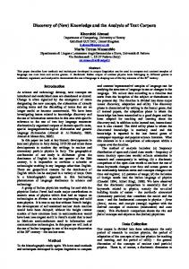
We used the anonymous Web data from www.microsoft.com created by Jack S. Breese, David Heckerman, and Carl M. Kadie from Microsoft. The data was created by sampling and processing the www.microsoft.com logs and donated to the Machine Learning Data Repository stored at University of California at Irvine Web site [8]. The Web log data keeps track of the use of Microsoft Web site by 38000 anonymous, randomly-selected users. For each user, the data records list all the areas of the Web sites that the user visited in a one week time frame. We used the training set only which has 32711 instances. Each instance represents an anonymous, randomly selected user of the Web site and corresponds to the transactions in market basket data. The number of attributes is 294 where each attribute is an area of the www.microsoft.com Web site and each attribute corresponds to an item in the store in the context of market basket data. We cleaned the data by removing the instances with less than or equal to non-zero attribute values and the resulting data set contained about 22k transactions. We have implemented the support reduction (GIH) and the first algorithm for confidence reduction (CR), using the Perl programming language. We have also implemented a naive Cyclic Hide (CH) algorithm that hides a rule by selecting the next transaction that supports the rule (in no particular order), and randomly replacing a 1 by a ? so the transaction no longer supports the item. The naive algorithm is used as a base for comparison with the rule and support reduction algorithms. As a first step, we run an Apriori based mining algorithm on the data with support 0.1%. We then obtained the rules out of the resulting large itemsets with 50% minimum confidence. The minimum confidence and support values are chosen with regard to typical minimum confidence and support thresholds from the literature. We then randomly selected 5 different (not necessarily disjoint) rules to test the hiding strategies. The selected rule set to be hidden is provided in Table 3. To assess the performance of the hiding strategies, we performed experiments on a 500MHz Pentium III PC with 512 MB of memory running the Linux operating system. In this exploratory study, we measured the CPU time requirement of the hiding strategies for different confidence values as depicted in Figure 4. As can be seen from the figure, all the hiding strategies hide the given rule set successfully in less than a second. That is considerably less than the time for mining of 57 seconds for 0.1% support. For various confidence values

confidence 76% 79% 83% 77% 53%

2. The same transaction could be modified in different ways to support different hidden rules – leading to discovery of hidden rules with too high support and confidence, and failure to discover others. This is even more likely if the rules are not disjoint.

How likely are these conditions in practice? Again, this is an area for future study. Perhaps the best way to combat this approach is to ensure that M ST , M CT , and SM are not known to the adversary. As M ST and M CT are likely fixed by the problem, the real key is to keep SM secret. Another way to combat rule/value reconstruction is to ensure that transactions have multiple unknowns corresponding to different real values, as discussed above. A challenge for the adversary we haven’t discussed is the computational complexity of reconstructing values. The first strategies (replace all ?s by 1s, then by 0s) are little more complex than finding rules without unknowns. The per-transaction heuristics are similar – compute support of all items, and one pass through the transactions with unknowns. The second approach is more complex. First, rules with low support and confidence must be discovered. Then, for each rule, all transactions have to be tested with either 1’s or 0’s to see the potential support and confidence. This is O(|D|) per rule. However, a simple change would greatly increase the complexity – instead of processing a rule with a single algorithm, interleave the algorithms between transactions in hiding a single rule (ensuring that CR2 is used as well as CR or GIH). Thus the adversary couldn’t just test by replacing all transactions with 1’s or 0’s – all possible combinations would need to be tried. This now becomes a O(2|D| ) problem. However, the potential side effects of such a strategy still need to be determined. 8

the GIH method (generating itemset support reduction algorithm Shown in Figure 1) and CH (Cyclic Hide) perform similarly while the CR (confidence reduction algorithm shown in Figure 2) hides the rules faster. However our main performance criterion of the different algorithms is the side effects they incur on the database. We measure the side effects by summing up the number of rules hidden unintentionally and the number of newly introduced rules. The performance of the hiding strategies in terms of the side effects are depicted in Figure 5. As can be observed from the figure, the CR causes the least number of side effects followed by GIR. CR and GIR outperform CH for all confidence values.

downgrade based upon the rules that it thinks Low can infer (i.e., by using decision tree analysis) and upon the importance of the information that Low should receive. Their objective then in developing this paradigm is to assign a penalty function to the parsimonious downgrading in order to minimize the amount of information that is not downgraded and to compare the penalty costs to the extra confidentiality that is obtained. Clifton [5] investigates the techniques to address the basic problem of using non-sensitive data to infer sensitive data in the context of data mining. His goal is to accomplish privacy by ensuring that the data available to the adversary is only a sample of the data on which the adversary would like the rules to hold. In addition, Clifton shows that for classification purposes, the security officer is able to draw a relationship between the sample size and the likelihood that the rules are correct. Agrawal and Srikant [2] investigate the development of a data mining technique that incorporates privacy concerns. In particular, they consider the concrete case of building a decision tree classifier from training data in that the values of individual records have been perturbed. Their goal is to use the perturbed data (acquired either by a discretization or by a value distortion technique) in order to accurately estimate the original distribution of the data values. By doing this, they are able to build classifiers whose accuracy is comparable to the accuracy of classifiers built with the original data. Agrawal and Aggarwal [1] improve on the distribution reconstruction technique presented in [2] by using the Expectation Maximization (EM) method. The authors claim that EM is more effective than the currently available technique in terms of the level of information loss. They also prove that EM converges to the maximum likelihood estimate of the original distribution based on the perturbed data and that it provides robust estimates of the original distribution. Finally, they propose novel metrics for the quantification and measurement of privacy-preserving data mining algorithms. A new class of privacy preserving techniques is introduced in [3, 9, 6]. In particular Atallah et. al [3], Dasseni et. al. [6] and Verykios et. al. [9] have considered the problem of privacy preserving mining of association rules. The authors have demonstrated how certain sensitive rules can be hidden by some data modification techniques and they have proposed efficient heuristics for solving this problem since Atallah et. al. [3] proved that the problem is NP-Hard. In the current work we are considering the same problem but instead of allowing random data modifica-

CPU Time For Different Hiding Strategies GIH CR CH

CPU time (secs)

0.6

0.4

0.2

0.0

10

20

30 Confidence (%)

40

50

Figure 4: CPU Performance Results Side Effects of Different Hiding Strategies

750

GIH CR CH

650

Side Effects

550 450 350 250 150 50

10

20

30 Confidence (%)

40

50

Figure 5: Side-effect Results

7

Related Work

The problem addressed in this paper is closely related to the inference problem in databases and the privacy preservation problem in data mining. Chang and Moskowitz [4] consider a solution of the database inference problem by using a new paradigm where decision tree analysis is combined with parsimonious downgrading. In their scheme, Chang and Moskowitz, propose that High decides what not to 9

tion, we have restricted ourselves to introducing ? a special symbol that indicates that information is missing. Some changes to the original association rule discovery program are necessary for the introduction of heuristics based on this idea.

8

[2] R. Agrawal and R. Srikant. Privacy Preserving Data Mining. Proceedings of SIGMOD Conference, pages 45–52, 2000. [3] M. J. Atallah, E. Bertino, A. K. Elmagarmid, M. Ibrahim, and V. S. Verykios. Disclosure Limitation of Sensitive Rules. Proceedings of IEEE Knolwedge and Data Engineering Workshop, pages 45–52, November 1999.

Conclusions

Sharing of data is often beneficial, but is often prevented because of privacy and security concerns. We have presented a technique to obscure a specific set of association rules, while minimizing the effect on the usefulness of the data for purposes other than learning those rules. This work is a first step. Although we have argued that the rules are truly safe from an attack by an adversary, we have yet to formally prove that safety. Our initial results indicate that deterministic algorithms for privacy preserving association rules are a promising framework for controlling disclosure of sensitive data and knowledge. In the near future, we will investigate how probabilistic and information theoretic techniques can also be applied to this problem. There are several areas in this field calling out for additional research. A few examples are:

[4] L. Chang and I. S. Moskowitz. Parsimonious Downgrading and Decision Trees Applied to the Inference Problem. Proceedings of the Workshop of New Security Paradigms, pages 82–89, 1999. [5] C. Clifton. Using Sample Size to Limit Exposure to Data Mining. Journal of Computer Security, 8(4), 2000. [6] D. Elena, V. S. Verykios, A. K. Elmagarmid, and E. Bertino. Hiding Association Rules by using Confidence and Support. To appear in the Proceedings of Information Hiding Workshop, 2001. [7] T. H. Hinke, H. S. Delugach, and R. P. Wolf. Protecting databases from inference attacks. Computers and Security, 16(8):687–708, 1997. [8] U. of California at Irvine Machine Learning Repository. http://www.ics.uci.edu/˜mlearn/MLSummary.html.

• More complete analysis of the effectiveness of these rule obscuring techniques, and formal study of the problem.

[9] V. S. Verykios, A. K. Elmagarmid, B. Elisa, D. Elena, and Y. Saygin. Association Rule Hiding. IEEE Transactions on Knowledge and Data Engineering, 2000. Under review.

• Other approaches to obscuring rules. • What happens with interest measures other than support and confidence? Is it possible that the sensitive rules are still likely to show up using, for example, a χ2 test? • Comparable work on other types of data mining. For example, what if the goal is to prevent the adversary from identifying clusters in the data? Being able to learn to classify data (or to classify specific subsets of items)? The grand goal should be to encourage the beneficial sharing of data, by ensuring that the shared data does not contain hidden “secrets”.

References [1] D. Agrawal and C. Aggarwal. On the Deisgn and Quantification of Privacy Preserving Data Mining Algorithms. Proceedings of PODS, pages 247–255, 2001. 10