Jan 15, 2014 - Peripheral (USRP) experimental results of the Max-Min signal .... min(A + B)αmin. αH. minBαmin. (4) max αmax. αH max(A + B)αmax. αH.
1
USRP Implementation of Max-Min SNR Signal Energy based Spectrum Sensing Algorithms for Cognitive Radio Networks
arXiv:1401.3407v1 [stat.AP] 15 Jan 2014
Tadilo Endeshaw Bogale and Luc Vandendorpe ICTEAM Institute, Universit`e catholique de Louvain Place du Levant, 2, B-1348, Louvain La Neuve, Belgium Email: {tadilo.bogale, luc.vandendorpe}@uclouvain.be
Abstract— This paper presents the Universal Software Radio Peripheral (USRP) experimental results of the Max-Min signal to noise ratio (SNR) Signal Energy based Spectrum Sensing Algorithms for Cognitive Radio Networks which is recently proposed in [1]. Extensive experiments are performed for different set of parameters. In particular, the effects of SNR, number of samples and roll-off factor on the detection performances of the latter algorithms are examined briefly. We have observed that the experimental results fit well with those of the theory. We also confirm that these algorithms are indeed robust against carrier frequency offset, symbol timing offset and noise variance uncertainty.
I. I NTRODUCTION The current wireless spectrum access strategy, which is fixed, utilizes the available frequency bands inefficiently [2], [3]. A promising approach of addressing this problem is to deploy a cognitive radio (CR) network. One of the key characteristics of a CR network is its ability to discern the nature of the surrounding radio environment. This is performed by the spectrum sensing (signal detection) part of a CR network. The most common spectrum sensing algorithms for CR networks are matched filter, energy, cyclostationary and eigenvalue based algorithms. As energy detector is simple to implement, several papers present experimental results of energy detector (see for example [4], [5]). The experimental results of these papers verify the existence of noise variance uncertainty. And, due to this reason, there is an signal to noise ratio (SNR) wall in which energy detector can not guarantee a certain detection performance. Recently new max-min SNR signal energy based spectrum sensing algorithms have been proposed in [1], [6]. Simulation results of these two papers show that the latter algorithms are robust against noise variance uncertainty, adjacent channel interference, carrier frequency offset and symbol timing offset. This motivate us proceed with the Universal Software Radio Peripheral (USRP) implementation of the spectrum sensing algorithms of [1], [6]. The remaining part of this paper is organized as follows: Section II discusses the hypothesis test problem. Section III presents the summary of the spectrum sensing algorithms The authors would like to thank SES for the financial support of this work, the french community of Belgium for funding the ARC SCOOP and BELSPO for funding the IAP BESTCOM project.
of [1], [6]. In Section IV, detailed experimental results are discussed. Finally, conclusions are drawn in Section V. Notations: The following notations are used throughout this paper. Upper/lower case boldface letters denote matrices/column vectors. The X(n,n) , X(n,:) , XT and XH denote the (n, n) element, nth row, transpose and conjugate transpose of X, respectively. In (I) is an identity matrix of size n × n (appropriate size) and, (.)⋆ , E{.}, |.| and (.)∗ denote optimal, expectation, absolute value and conjugate operators, respectively. II. P ROBLEM FORMULATION Assume that the transmitted symbols sn , ∀n are pulse shaped by a filter g(t). After the digital to analog converter, the base band transmitted signal is given by ∞ ∑ x(t) = sk g(t − kPs ) (1) k=−∞
where Ps is the symbol period. In an additive white Gaussian noise (AWGN) channel, the base band received signal is expressed as ∫ ∞ r(t) = f ∗ (τ )(x(t − τ ) + w(t − τ ))dτ =
∫
=
∞
−∞
f ∗ (τ )(
−∞
∞ ∑
k=−∞
∞ ∑
k=−∞
sk g(t − kPs − τ ) + w(t − τ ))dτ
sk h(t − kPs ) +
∫
∞
−∞
f ∗ (τ )w(t − τ )dτ
where f ∗ (t) is the receiver filter, ∫ ∞ w(t) is the additive white Gaussian noise and h(t) = −∞ f ∗ (τ )g(t − τ )dτ . The objective of spectrum sensing is to decide between H0 and H1 from r(t), where ∫ ∞ r(t) = f ⋆ (τ )w(t − τ )dτ, H0 (2) =
∞ ∑
−∞
k=−∞
sk h(t − kPs ) +
∫
∞
−∞
f ⋆ (τ )w(t − τ )dτ, H1 .
Without loss of generality, we assume that r(t) is a zero mean signal. Note that when r(t) has a nonzero mean, its mean can be removed before examined by the proposed spectrum sensing algorithms.
III. S UMMARY OF THE SPECTRUM SENSING ALGORITHMS OF [1], [6] The main idea of the algorithms of [1], [6] is to apply linear combination approach for the oversampled received signal. These papers consider that the transmit pulse shaping filter is assumed to be known. Under this assumption, the linearly combined signal {˜ y [n]}N n=1 can be expressed as [1], [6] y˜[n] , =
L−1 ∑
αi r((n − 1)Ps + ti )
i=0 ∞ ∑
sk
i=0
k=−∞ L−1 ∑ i=0
αi
L−1 ∑
∫
∞
−∞
(3)
αi h((n − 1)Ps + ti − kPs )+
f ⋆ (τ )w((n − 1)Ps + ti − τ )dτ
{ti }L−1 i=0
where are chosen such that tL −t0 = Ps and {αi }L−1 i=0 are the introduced variables. For the given g(t) (of course f (t) is always known as it is designed by the cognitive receiver), the optimal {αi }L−1 i=0 that minimize and maximize the SNR of y˜[n] can be obtained by solving the following optimization problems: αH min (A + B)αmin (4) αmin αH min Bαmin αH (A + B)αmax (5) max maxH αmax αmax Bαmax ∑∞ ′ ⋆ ′ where A(i+1,j+1) ∫ ∞ = ⋆ k′ =−∞ h(k Ps + ti )h (k Ps + tj ) and B(i+1,j+1) = −∞ f (τ )f (ti − tj + τ )dτ As these two problems are Rayleigh quotient, the optimal solutions of these problems can be found by the Generalized Eigenvalue solution approach. Using these solutions, the following test statistics is proposed [1], [6]: √ b (6) T = N (Te − 1). min
where
∑N ∑N ca2z y [n]|2αmax |z[n]|2 M be n=1 |˜ T = ∑N , , ∑n=1 N 2 ca2e y [n]|2αmin M n=1 |˜ n=1 |e[n]|
N N ∑ ∑ ca2z = 1 ca2e = 1 M |z[n]|2 , M |e[n]|2 . N n=1 N n=1
The Pf and Pd of this test statistics are obtained by applying asymptotic analysis and are given as ( ) λ Pf (λ) =P r{T > λ|H0 } = Q (7) σ ˜ ( H0 ) λ−µ Pd (λ) =P r{T > λ|H1 } = Q (8) σ ˜H1 √ where λ is the threshold, µ = N 1+γγdmin , γmin /γmax is the SNR obtained by solving (4)/(5), γd = γmax − γmin , 2 2 σ ˜H0 (˜ σH1 ) is the variance of (6) under H0 (H1 ) hypothesis and Q(.) is the Q-function which is defined as [7] ∫ ∞ x2 1 exp− 2 dx. Q(λ) = √ 2π λ
As can be seen from (4) and (5), for a given g(t), the achievable maximum and minimum SNRs depend on the selection of f (t), L and {ti }L−1 i=0 . As discussed in [1], [6], for a given g(t), getting the optimal f (t), L and {ti }L−1 i=0 ensuring the highest detection performance is an open research topic. In this experiment, we select f (t), L and {ti }L−1 i=0 as in [1], [6] (i.e., f (t) = g(t) (i.e., matched filter), L = 8 and {ti = Ps ( 21 + Li )}L−1 i=0 ). From the above explanation, one can realize that to get the Pd of (8), t0 must be known perfectly. The exact t0 is known when the receiver is synchronized perfectly with the transmitter. However, in general, since the transmitters and receivers are controlled by different network operators, perfect synchronization is not possible. From (3), we can notice that there are L possible values of y˜[n]. Consequently, we will have L possible values of T (i.e., (6)). Therefore, for asynchronous receiver scenario, one naive approach of adapting the detection algorithm of (6) is just to choose any of {Ti }L i=1 randomly (i.e., detection algorithm without estimation of t0 ). The other approach is that under H0 hypothesis, all values of {Ti }L i=1 are almost the same, whereas, under H1 hypothesis, the values of {Ti }L i=1 are not the same. And, the t0 corresponding to Tmax = max[T1 , T2 , · · · , TL ] can be considered as the best estimate of the true t0 . Due to this reason, the following test statistics is proposed (i.e., detection algorithm with estimation of t0 ) [1]: Tmax = max[T1 , T2 , · · · , TL ].
(9)
The Pf and Pd of the asynchronous receiver with and without estimation of t0 test statistics can be obtained in [1]. IV. E XPERIMENTAL RESULTS In this section, we provide experimental results. The experiment is conducted in an indoor wireless environment as shown in Fig. 1. The air distance between the transmitter and receiver is around 8m. For the experiment, we use National Instruments USRP (NI-USRP) and employ a LabVIEW 2012 version software. The carrier frequency of the transmitted signal is set to 433.5MHz which is the industrial, scientific and medical (ISM) band of Europe [8]. All of the experimental results of this section are obtained by averaging 10000 realizations.The SNR is defined σ2 as SN R , σ2s which is estimated from the received signal w (i.e., from the average powers under H0 and H1 hypothesis). For this experiment, we consider an orthogonal frequency division multiplexing (OFDM) transmitted signal with the parameters as shown in Table I. The transmitted signals are pulse shaped by a square root raised cosine filter (SRRCF) with a roll-off factor 0.2, 0.25 or 0.35. The receiver employs a matched filter (i.e., SRRCF) and Nd = N = 215 . Under this assumption and asynchronous receiver (with and without estimating t0 detection) scenarios, the coefficients of α and the thresholds that achieve Pf ≤ 0.1 are presented in Appendix A. In all of the figures, ”Async with (w/o) est” represents asynchronous receiver with (without) estimation of t0 scenario, and ”Exp”, ”Sim” and ”The” denote experimental, simulation and theoretical results, respectively.
TABLE I E XPERIMENTAL PARAMETERS OF TRANSMITTED OFDM SIGNAL Parameter Channel BW FFT size (NF F T ) Used subcarrier index Cyclic prefix (CP) ratio Modulation per OFDM symbol Pulse shaping filter
Value 625 KHz 256 {-120 to 1 & 1 to 120} 1/8 QPSK SRRCF with rolloff 0.2
Pf curve for SRRCF with rolloff=0.2
1
Async w/o est (The) Async w/o est (Exp) Async with est (The) Async with est (Exp)
0.9 0.8 0.7 0.6 Pf
Fig. 1. The experimental environment (University Catholique de Louvain (UCL) Lab).
0.5 0.4 0.3
Normalized Power Spectral Density 0
0.2 0.1
−10 Desired band
0 −6 −5 −4 −3 −2 −1
PSD (in dB)
−20
4
5
6
7
8
−30
Fig. 3.
−40
Theoretical versus experimental Pf results.
−50
A. Pre-processing of the received signal
−60 −70 −80 −0.5 −0.4 −0.3 −0.2 −0.1 0 0.1 0.2 Frequency (in F )
0.3
0.4
0.5
0.4
0.5
s
(a) Normalized Power Spectral Density 0 −10 −20 PSD (in dB)
0 1 2 3 Threshold (λ)
New position of the desired band
−30 −40 −50 −60 −70 −80 −0.5 −0.4 −0.3 −0.2 −0.1 0 0.1 0.2 Frequency (in F )
0.3
s
(b) Fig. 2. Sample spectrum taken from the NI-USRP under H0 hypothesis with carrier frequency 432.25MHz and IQ sampling rate (Fs ) of 5M: a) Spectrum of the received signal. b) Spectrum of the pre-processed signal.
According to [9], the Analog to Digital Converter (ADC) of the NI-USRP has a maximum spurious free dynamic range of 88dB. Consequently, some of the received signals may be clipped. Due to this and local oscillator drift, this USRP will have strong spur in the low frequency regions (see Fig. 2.(a)). This spur, of course, is not a true transmitted signal and therefore should be handled properly. From several observations of the received signal under H0 hypothesis, we have realized that the maximum width of this spur is F8s Hz (i.e., it covers at most [- F16s F16s ] bands), where Fs is the In phase and Quadrature (IQ) sampling rate of the USRP. And since the algorithm of [1] employs oversampling of the received signal by a factor of 8 (i.e., the band which we want to examine has a double-sided bandwidth of F8s ), it is possible to shift the spurious data bands to the undesired band. This can be performed easily by multiplying the received signal s with exp−jωt . In this experiment, we choose ω = πF 2 (see Fig. 2.(b)). In the following, we examine the performance of the algorithms of [1] for the pre-processed signal. B. Verification of the Pf curve In this experiment, we verify the theoretical versus experimental Pf curves of the algorithms of [1]. Fig. 3 shows the theoretical and experimental Pf curves. From this figure, we can notice that the experimental Pf curves match well with those of the theoretical ones.
1 0.9
0,84
Async w/o est (Exp) Async with est (Exp) 2
Async w/o est (Sim AWGN ∆σ =0) 0.8
Async w/o est (Sim AWGN ∆σ2=2dB) Async with est (Sim AWGN ∆σ2=2dB)
0,75
Async w/o est Async with est
d
0.6
P
Pd
0.7
0,8
Async with est (Sim AWGN ∆σ2=0)
0,7
0.5 0.4
0,65
0.3 0.2
−19
−18
−17 SNR
−16
−15
−14
Fig. 4. Experimental and simulation Pd results for different SNR values when roll-off=0.2. In this figure, ∆σ 2 denotes the noise variance uncertainty as defined in [1].
0.0156
0.1406 Cyclic prefix (CP)
0.2031
0.25
Fig. 5. Experimental Pd results for different transmitted signal cyclic prefix ratios when roll-off=0.2 and SNR=-13.8dB.
C. Effect of SNR
0.9 0.8 0.7 0.6 Pf (Pd)
In this subsection, we examine the Pd of the algorithm of [1] for different SNR values as shown in Fig. 4. As we can see from this figure, the Pd of the algorithm of this paper increases as the SNR increases. Moreover, we can notice that the experimental channel is closer to the AWGN channel which is expected. This is due to the fact that the transmitter and receiver are placed in a static position and there is a line of sight between the transmitter and receiver (see Fig. 1). Thus, the experimental environment can be modeled as an AWGN channel.
0.0781
0.5
Pd (Async w/o est) Pd (Async with est) Pf (Async w/o est) Pf (Async with est) Target P
0.4 0.3
f
0.2 0.1
D. Effect of cyclic prefix In this subsection, we consider the effect of the transmitted signal cyclic prefix (CP) on the performance of the algorithms. Fig. 5 shows the performance of the detection algorithms of [1] 1 1 1 for practically relevant CP factors (i.e., 14 , 18 , 16 , 32 , 64 ). From this figure, we can understand that the detection probabilities of the latter algorithms are almost the same for different transmitted signal CP factors.
0 1
2 3 Number of samples (in N )
4
d
Fig. 6. Experimental Pd (Pf ) results for different number of samples (Nd ) when roll-off=0.2 and SNR=-15.9dB.
0,9 0,8
E. Effect of Nd
0,7 0,6 Pd(Pf)
Here the effect of Nd on the performances of the algorithms of [1] is examined. As we can see from Fig. 6, the Pd of these algorithms increase as Nd increases and the algorithms also maintain the desired Pf for all values of Nd .
Pd (Async w/o est) Pd (Async with est) Pf (Async w/o est) Pf (Async with est) Target P
0,5 0,4
F. Effect of roll-off factor
0,3
In this experiment, we examine the effect of the roll-off factor on the detection performance of the algorithms of [1] which is shown in Fig. 7. As can be seen from this figure, the Pd of the latter algorithms increase as the roll-off factor increase and the Pf s are maintained for all roll-off factors. From the Figs. 3 - 7, we can notice that all the experimental Pd and Pf results are in agreement with the theoretical ones. And the performance of all experiments are closer to
0,2
f
0,1 0.2
0.25
0.3
0.35
Rolloff factor
Fig. 7. Experimental Pd (Pf ) results for different roll-off factors when SNR=-13.8dB.
TABLE II T HE THRESHOLD (λ FOR Pf ≤ 0.1) AND THE COEFFICIENTS OF α: I N THIS TABLE , β DENOTES THE ROLLOFF FACTOR AND λw (λw/o ) IS THE THRESHOLD TO ENSURE
Pf ≤ 0.1 FOR
THE ASYNCHRONOUS SCENARIO
WITH ( WITHOUT ) ESTIMATION OF t0 .
β λw/o λw α
0.2 2.96 4.586 αmin -8.8565 5.2981 8.3685 3.8283 -3.4689 -8.1746 -5.4128 8.3317
αmax -0.0586 -0.0033 0.1166 0.2486 0.3346 0.3213 0.1697 -0.1375
0.25 2.925 4.525 αmin -8.1340 4.8609 7.7102 3.5405 -3.1840 -7.5180 -4.9741 7.6169
αmax -0.0585 -0.0036 0.1164 0.2488 0.3350 0.3214 0.1692 -0.1374
0.35 2.75 4.22 αmin -6.6562 3.9772 6.3653 2.9492 -2.6034 -6.1790 -4.0856 6.1629
αmax -0.0581 -0.0044 0.1158 0.2492 0.3361 0.3217 0.1682 -0.1374
that of the theoretical AWGN channel environment scenario of [1] for both asynchronous with and without estimating t0 detection scenarios. Also, since we employ two separate USRP and desktop computers without clock synchronization and the knowledge of noise variance, we can notice that the algorithms of [1] are indeed robust against carrier frequency offset, symbol timing offset and noise variance uncertainty. This shows that these algorithms can be applied for practical spectrum sensing algorithms. Note that since the SNR of the experimental result is estimated from the received signal, the SNR of the current paper is not accurate. Due to this fact, the Pd shown in Fig. 4 is not exactly the same as that of the AWGN channel. V. C ONCLUSIONS This paper discusses the experimental results of the spectrum sensing algorithms of [1]. For the experiment, we apply NI-USRP hardware with LabVIEW 2012 software. The experiment is conducted for different parameter settings. In particular, we examine the effects of SNR, CP, Nd and rolloff factor on the Pd (and Pf ) of the algorithms of the latter paper. Experimental results show that these algorithms ensure the desired Pf (Pd ) for the aforementioned parameter settings. Also, the experimental results demonstrate that these algorithms are indeed robust against carrier frequency offset, symbol timing offset and noise variance uncertainty. A PPENDIX A In the current paper, we employ the linear combination coefficients (α) and threshold (λ) as shown in Table II. R EFERENCES [1] T. E. Bogale and L. Vandendorpe, “Max-Min SNR signal energy based spectrum sensing algorithms for cognitive radio networks with noise variance uncertainty,” IEEE Tran. Wirel. comm, 2013. [2] I. F. Akyildiz, W. Lee, M. C. Vuran, and S. Mohanty, “Next generation/dynamic spectrum access/cognitive radio wireless networks: A survey,” Journal of Computer Networks (ELSEVIER), vol. 50, pp. 2127 – 2159, 2006. [3] M. Nekovee, “A survey of cognitive radio access to TV white spaces,” International Journal of Digital Multimedia Broadcasting, pp. 1 – 11, 2010.
[4] D. Cabric, A. Tkachenko, and R. W. Brodersen, “Experimental study of spectrum sensing based on energy detection and network cooperation,” in Proceedings of the first international workshop on Technology and policy for accessing spectrum, New York, NY, USA, 2006, TAPAS ’06, ACM. [5] H. Kim, C. Cordeiro, K. Challapali, and K. G. Shin, “An experimental approach to spectrum sensing in cognitive radio networks with offtheshelf,” in IEEE 802.11 Devices, in IEEE Workshop on Cognitive Radio Networks, in conjunction with IEEE CCNC, 2007. [6] T. E. Bogale and L. Vandendorpe, “Linearly combined signal energy based spectrum sensing algorithm for cognitive radio networks with noise variance uncertainty,” in 8th International Conference on Cognitive Radio Oriented Wireless Networks (CROWNCOM), Washington DC, USA, 8 – 10 Jul. 2013. [7] none, “Q-function,” http://en.wikipedia.org/wiki/ Q-function. [8] M. Engjom, “Using the CC1100/CC1150 in the European 433 and 868 MHz ISM bands,” in Texas Instrument, Application Notes AN039. [9] none, “National instruments universal software peripheral (NI-USRP) documentation,” http://www.ni.com/pdf/manuals/375987a. pdf.