Utility of the Wavelet Transform for LAI Estimation Using Hyperspectral Data Asim Banskota, Randolph H. Wynne, Shawn P. Serbin, Nilam Kayastha, Valerie A. Thomas, and Philip A. Townsend
Abstract
We employed the discrete wavelet transform to reflectance spectra obtained from hyperspectral data to improve estimation of LAI in temperate forests. We estimated LAI for 32 plots across a range of forest types in Wisconsin using hemispherical photography. Plot spectra were extracted from AVIRIS data and transformed into wavelet features using the Haar wavelet. Separately, subsets of spectral bands and the Haar features selected by a genetic algorithm were used as independent variables in linear regressions. Models using wavelet coefficients explained the most variance for both broadleaf plots (R2 = 0.90 for wavelet features versus R2 = 0.80 for spectral bands) and all plots independent of forest type (R2 = 0.79 for wavelet features vs. R2 = 0.58 for spectral bands). The forest-type specific models were better than the models using all plots combined. Overall, wavelet features appear superior to band reflectances alone for estimating temperate forest LAI using hyperspectral data.
Introduction
Leaf area index (LAI) of vegetation canopies controls and moderates different climatic and ecological functions (Gong et al., 1995; Huemmrich et al., 2005; Leblanc and Chen, 2001). In forests, LAI determines light interception and thereby CO2 fixation, canopy photosynthesis, and stand productivity (Turner et al., 2003). It affects hydrological processes and litter production and thus the dynamics of soil water and nutrient cycling (Oren et al., 1998). As such, most ecosystem process models that simulate carbon and hydrologic cycles require LAI as an input variable (Gower, 2001). LAI is one of the principal factors controlling canopy reflectance (Asner, 1998). However, LAI alone cannot fully describe the effects of canopy structure on reflectance as canopies with similar LAI often have significantly different near infrared (NIR) reflectance (Ollinger, 2011). As such, a large body of research has investigated the use of airborne and satellite remote sensing data for its accurate estimation (Fassnacht et al., 1997; Gong et al.,
Asim Banskota is with School of Forest Resources and Environmental Science, Michigan Tech, Houghton, Michigan, and formerly with Department of Forest Resources and Environmental Conservation, Virginia Polytechnic Institute and State University, Blacksburg, Virginia (
[email protected]). Randolph H. Wynne, Nilam Kayastha, and Valerie A. Thomas are with Department of Forest Resources and Environmental Conservation, Virginia Polytechnic Institute and State University, Blacksburg, Virginia. Shawn P. Serbin and Philip A. Townsend are with Department of Forest and Wildlife Ecology, University of WisconsinMadison, Madison, Wisconsin. PHOTOGRAMMETRIC ENGINEERING & REMOTE SENSING
1995; Huemmrich et al., 2005; Ilames et al., 2008; Jensen et al., 2012). The most widely used approach is to establish an empirical relationship between LAI measured in situ and spectral vegetation indices (SVIs) calculated from spectral reflectance in two or three bands (Haboudane et al., 2004). However, most empirical approaches are limited in application because the relationship between LAI and SVIs saturates at dense canopy conditions characterized by high LAI (Broge and Leblanc, 2000). The other shortcoming is that SVIs are sensitive to many different factors apart from variation in LAI, such as variation in leaf optical properties and background spectral reflectance (Goward et al., 1994). Hyperspectral sensors enable measurement of surface reflectance in narrow spectral bands, providing a capability to analyze canopy by absorption features and over a near continuous spectrum (Asner, 1998; Pu et al., 2008; Thenkabail et al., 2002). Both the absorption features and overall shape of the reflectance curve have been found to be sensitive to variability in LAI (Asner, 1998). Darvishzadeh et al. (2008) and Lee et al. (2004) found that the relationship between measured and estimated LAI can be better explained by multiple regression using a combination of narrow bands from imaging spectroscopy (hyperspectral) data than univariate methods using narrow band SVIs. However, one of the major caveats of using hyperspectral imagery is the greater noise and correlation among spectral bands. Statistical models can suffer from multi-collinearity (Geladi and Kowalski, 1986) and overfitting (Coops et al., 2003) when a large number of redundant bands are used as predictive variables. Hence, effective use of hyperspectral data for empirical estimation of LAI requires reduction of dimensionality. Such data reduction also leads to the loss of useful features offered by spectroscopic data, such as information about the overall shape of a reflectance continuum, as well as gradual and abrupt slope changes between neighboring bands. The wavelet transform, a signal processing technique, has become increasingly important to numerous vegetation-related applications of hyperspectral remote sensing (Banskota et al., 2011; Blackburn, 2007; Blackburn and Ferwerda, 2008; Bruce et al., 2001; He et al., 2012; Pu and Gong, 2004; Ranchin et al., 2001; Wang, 2010; Zhang et al., 2006). The wavelet transform reduces the dimensionality of hyperspectral data by projecting them into a new feature space in which just a few wavelet coefficients represent most of the information in the original data. Wavelet representation of hyperspectral data also conveys additional information such as the location and nature of
Photogrammetric Engineering & Remote Sensing Vol. 79, No. 7, July 2013, pp. 653–662. 0099-1112/13/7907–653/$3.00/0 © 2013 American Society for Photogrammetry and Remote Sensing July 2013
653
high frequency features (narrow absorption features, red-edge inflection point, and noisy bands), and the magnitude and shape of the reflectance continuum at different scales and positions (Banskota et al., 2011). Pu and Gong (2004) compared wavelet “energy features” (Bruce et al., 2001; Zhang et al., 2006) from Hyperion hyperspectral imagery to the original spectral bands and principal components to estimate LAI. Although the energy features approximate the partitioning of the energy across multiple scales, the features do not provide any measure of the energy distribution at specific wavelength positions. For vegetation applications in particular, the latter is more critical because the coefficients related to specific wavelength regions of hyperspectral data resolved at different scales might be more useful than coefficients related to other regions and scales. Banskota et al. (2011) found energy features performed poorly compared to both spectral bands and wavelet coefficients for pine species discrimination. Similar to species discrimination, narrow band reflectance at some specific wavelength regions (such as red-edge and NIR water absorption regions) have been found to be greatly sensitive to variation in LAI (Asner, 1998). As such, this study focuses on the selection of the appropriate coefficients to better utilize the wavelet transform for estimating LAI. Our principal objective was to determine whether empirical estimation of LAI using hyperspectral data can be improved by using Haar wavelet coefficients rather than the original spectral bands as the independent variables. Additionally, we wished to identify the wavelet coefficients that provide the best LAI estimates in diverse temperate forest types.
Background on Wavelet Transforms
A wavelet transform enables signal (data) analysis at different scales or resolutions by creating a series of shifted and scaled versions of the mother wavelet function (Banskota et al., 2011; Hsu, 2007). The term “mother” implies that a set of basis functions {Ca,b(λ)} can be generated from one main function, or the mother wavelet C(λ) by the following equation (Bruce et al., 2001):
(
)
(1) ψ a ,b ( λ ) = 1 ψ λ – b . a a where a is the scaling factor of a particular basis function, and b is the translation variable along the function’s range. In this study, we employ the Haar wavelet transform (DWT), which separates a discrete signal f of length n into two subsignals, each with length n/2, one being a running average and the other a running difference (Walker, 1999). We refer to the running average, or trend, as the approximation vector, a. For each m = 1, 2, 3,…, n/2, the approximation coefficient is calculated as: f f (2) am = m 1 2 m . 2 We refer to the running difference, or fluctuation, as the detail vector, d. Each of the detail coefficients is calculated as: f f (3) dm = m 1 2 m . 2 The sub-signals of the original signal define the first level of the Haar transform, usually referred to as 1-level. As such, the approximation coefficients and detail coefficients from the first level can be referred to as a1 and d1, respectively. Computation of approximation and detail coefficients for subsequent levels is achieved by recursively applying Equations 2 and 3 to the approximation coefficients of the previous level. Since the sub-signals have half the length of the previous signal, a2 and d2 will have half the length of a1, or n/4. The number of times n is divisible by two yields the 654 J u l y 2 0 1 3
possible number of decomposition levels. For example, if n = 16 = 24, four levels of Haar transforms can be computed. Mallat (1989) developed an efficient way to implement the Haar DWT scheme by representing the wavelet basis as a dyadic filter tree, or set of high-pass and low-pass filters. The highpass and low-pass filters are related (their power sum is equal to one) and called quadrature mirror filters. Thus, the 1-level DWT decomposition of a signal splits it into a low pass version (approximation coefficients) and a high pass version (detail coefficients). The 2-level decomposition is performed on the low pass signal obtained from the first level of decomposition. The final results of a DWT decomposition of a spectrum are sets of wavelet coefficients, with each wavelet coefficient directly related to the amount of energy in the signal at different positions in the spectrum and at different scales.
Background to Genetic Algorithms
The genetic algorithm (GA; Holland, 1975) is used to solve optimization problems. In the process of variable selection, the “fitness” of random subsets of potential variables can be assessed similar to Darwin’s biological theory of “natural selection” and “survival of the fittest” (Lin and Sarabandi, 1999) in which more genetically fit individuals have a greater chance of selection. Subsets with greater fitness are allowed to survive and undergo exchange of variables. A genetic algorithm is initialized with input parameters and a random population of a subset of variables. Each subset is assessed according to a specified fitness function (e.g., goodness of fit), with subsets performing below the average fit discarded. When the population of variables is shrunk to half its original size, the genetic algorithm cross-breeds the retained subsets of variables to replace the discarded subsets. The population of variables returns to the original size and the process continues again at the fitness evaluation step. The entire process stops once a predefined criterion is met or convergence is reached and best subset of identified variables is returned. Genetic algorithms have been found useful for selecting variables for different remote sensing applications (Kooistra et al., 2003; Luo et al., 2003; Vaiphasa et al., 2007).
Methods Study Area The study area comprises a range of coniferous, broadleaf deciduous, and mixed forest types across different ecoregions within the state of Wisconsin (Figure 1). The northern-most forest sites were located within the Northern Lakes and Forest ecoregion and Chequamegon-Nicolet National Forest, near Park Falls, Wisconsin, which is dominated by a mixed-hardwood forest originating from large-scale clear-cut practices of the early twentieth century (Curtis, 1959). The overstory vegetation was comprised mostly of northern hardwoods dominated in the uplands by sugar maple (Acer saccharum), basswood (Tilia americana), quaking aspen (Populus tremuloides), and white ash (Fraxinus americana); and in the lowlands by speckled alder (Alnus incanta), black ash (Fraxinus nigra) and red maple (Acer rubrum). The dominant coniferous species are balsam fir (Abies balsamea), white pine (Pinus strobus), red pine (Pinus resinosa), tamarack (Larix laricina), and black spruce (Picea mariana). The southern sites were located in the Baraboo Hills of the “Driftless” (unglaciated) ecoregion of Wisconsin. Most of the forests in the Baraboo Hills were cleared by the 1870s and have since recovered to forests dominated by red oak (Quercus rubra), white oak (Quercus alba), green and white ash (F. pennsylvanica and F. americana), hickories (Carya spp.), sugar maple, red maple, and basswood. PHOTOGRAMMETRIC ENGINEERING & REMOTE SENSING
(a)
(b1)
(b2)
(b3)
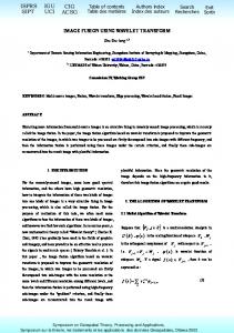
Figure 1. Study area: (a) State of Wisconsin showing general location of the three field sites, and (b) plot locations overlaid on a grey scale AVIRIS image.
LAI Measurement Protocol Optical measurements of effective LAI (Le) were estimated from hemispherical photos collected at one meter above the forest floor using a Nikon CoolPix 5000 digital camera, leveled on a tripod with an attached Nikon FC-E8 183° lens (Chen et al., 2006; Leblanc et al., 2005). Le represents the equivalent leaf area of a canopy with a random foliage distribution to produce the same light interception as the true LAI (Fernandes et al., 2004) and is derived from the canopy gap fraction at selected zenith angles beneath the canopy following Leblanc and Chen (2001): L LAI = e ( – ! ). (4) Ω where Le is the effective LAI, V is the clumping index and a is the woody-to-total leaf area ratio (a = W/Le (1/V)), in which W represents the woody-surface-area-index (half the woody area per m2 of ground area). In this study, we calculated LAI from Le by correcting the effect of clumping but neglecting the effect of woods and branches in Equation 4 (i.e., LAI = Le /V). This form of LAI was employed instead of Le because the clumping correction (especially for conifers) facilitated better relative estimates of LAI among vegetation types. Hemispherical images were collected at 33 plots (60 m × 60 m) characterized by broadleaf (18 plots), coniferous (11 plots), and mixed (4 plots) forest types. All measurements were made during the peak of the summer PHOTOGRAMMETRIC ENGINEERING & REMOTE SENSING
growing seasons in 2008 and 2010 during uniformly overcast skies or during dusk or dawn when the sun was hidden by the horizon. The measurements for majority of the broadleaf plot estimates were collected in 2008 (82 percent). We did not find any large differences in LAI for similar forest types collected in 2008 and 2010. None of our plots experienced any significant disturbances, and we did not expect any significant changes in LAI for these sites over two years. Images were collected in the JPEG format at the highest resolution (2560 × 1920 pixels) to maximize the detection of small canopy gaps (Leblanc et al., 2005). At each plot, we measured Le at nine subplot locations: the plot center, 30 meters from the plot center in each of the four cardinal directions, and the mid-point of each 30 m transect. Images were processed using DHP-TRAC software (Leblanc et al., 2005) to estimate Le and V, using a nine ring configuration but selecting only the first six rings for analysis to minimize the impacts of large zenith angles on the Le retrievals and the calculation of LAI (Chen et al., 2006; Leblanc et al., 2005). Descriptive statistics for plot LAI are given in Table 1.
AVIRIS Image Processing
Airborne Visible/Infrared Imaging Spectrometer (AVIRIS) data used in this study (Flight ID: f080713t01 and f080714t01) were acquired in July 2008 on NASA’s ER-2 aircraft at an altitude of 20 km, yielding a pixel (i.e., spatial) resolution of
July 2013
655
TABLE 1. GENERAL DESCRIPTIVE STATISTICS OF LAI ACCORDING TO VEGETATION FUNCTIONAL TYPES Plot type All Broadleaf Coniferous Mixed
N 33 18 11 4
Mean 4.65 5.00 4.02 4.61
Min 2.17 2.99 2.17 4.16
Max 6.67 6.67 5.62 5.37
∑ 0.92 0.80 1.00 0.50
approximately 17 m (16.8 to 17.0 m). The AVIRIS instrument produces 224 spectral bands (or wavelengths), with an approximate full-width half-maximum of 10 nm for each wavelength over the spectral range of 370 to 2500 nm (Green et al., 1998). AVIRIS image preprocessing involved manual delineation of clouds and cloud-shadows, cross-track illumination correction, and conversion to top-of-canopy (TOC) reflectance using atmospheric correction. Redundant bands between detectors were also removed. Cross-track illumination effects arise from a combination of flight path orientation and relative solar azimuth. We removed this effect by developing band-wise bilinear trend surfaces, ignoring all cloud/shadow-masked pixels, and trend-normalizing the images by subtracting the illumination trend surface and adding the image mean. Atmospheric correction of the cross-track illumination corrected images to TOC reflectance employed the ACORN5b™ software (Atmospheric CORrection Now; Imspec LLC, USA). Due to the low ratio of signal to noise at both spectral ends (366 nm to 395 nm and 2467 nm to 2497 nm), and in bands around the major water absorption regions (1363 nm to 1403 nm and 1811 nm to 1968 nm) those wavelength regions were dropped, resulting in a final total of 184 bands. The pixel spectra corresponding to the centers of the plot locations were extracted for the final 184 atmospherically corrected AVIRIS channels. One broadleaf plot of our 33 total was removed from the analysis based on Cook’s Distance, which identifies influential observations on the basis of how a linear function changes when a certain observation is deleted (Cook, 1979). The removed plot had the highest LAI (6.67) and unusually low reflectance throughout the near-infrared (NIR) region (maximum reflectance of 42 percent at NIR plateau). Cook’s test identified the plot as suspicious (partial F-statistic = 0.83; Cook’s distance = 0.97), and the reason for the discrepancy of this one plot was indeterminate, but likely due to either GPS error or disturbance to the plot between the times of data collection and imaging. Calculation of Discrete Wavelet Coefficients The DWT was implemented in Matlab (version 7.4; The Mathworks, Inc.) using a dyadic filter tree as previously discussed. The hyperspectral signal in the spectral domain extracted for each pixel location was passed through a series of low pass and high pass filters related to Haar wavelets. We chose the Haar mother wavelet as it is the simplest of all available wavelets, and recent investigations have illustrated its effectiveness for feature extraction of hyperspectral data (Bruce et al., 2001; Li, 2004; Zhang et al., 2006). The decomposition level was chosen such that it was maximized (6 for 184 bands using the Haar wavelet). All the detail wavelet coefficients calculated at each level and approximation coefficients at final level were concatenated to produce a final wavelet dataset. Variable Selection by GA The genetic algorithm employed the GA toolbox in Matlab (version 7.1; Mathworks, Inc.). The algorithm was run
656 J u l y 2 0 1 3
separately for two datasets (combined plots and only broadleaf plots) to find optimum subsets of features out of two different sets of variables: (a) original spectral bands, and (b) wavelet coefficients. Since the sample size for coniferous (11 plots) and mixed plots (4 plots) were low, we decided to analyze for broadleaf plots only for a single vegetation type analysis. For the fitness function, we used leave-one-out cross-validation (CV-RMSE) between observed LAI and estimated LAI. We used GA to find the optimal subset of variables that minimized the fitness function for different numbers of features (two to six). To avoid multicollinearity, the CV-RMSE was set to one for subsets with highly correlated variables (correlation coefficient greater than 0.8), ensuring that their fitness was minimized. The GA was run five times for each dataset to find the best subsets, with GA parameters (a) population = 100, (b) mutation rate = 0.5, (c) cross over rate = 0.5, and (d) stopping criterion = 100 generations or 25 generations with no improvement in the best fitness value. Statistical Analysis We used multiple linear regression to predict LAI as a function of the wavelet variables and spectral bands. Two subsets of variables were used as independent variables in both the analysis of all plots and the analysis using exclusively broadleaf plots: (a) wavelet coefficients selected by GA, and (b) spectral bands selected by GA. Selected models were subject to the following constraints: (a) all independent variables were significant at a = 0.05, and (b) there could not be multicollinearity, i.e., all variance inflation factors (VIFs) had to be less than 10. Consideration was also given to model parsimony, i.e., a model with fewer variables was preferred to one with many variables. To ensure the assumptions of multiple regression analysis were met, the regression residuals for all selected models were tested for normality using the Lilliefors test (Lilliefors, 1969). Leave-one-out cross validation was then used to evaluate the best models. The cross-validation coefficient of determination (CV-R2) and cross-validation RMSE (CV-RMSE) were calculated to assess the prediction capabilities of the best models. The confidence intervals for the regression statistics for best models were calculated using a bootstrap procedure in Matlab (version 7.4; The Mathworks, Inc.). The bootstrap method involves resampling of the original data in order to generate a distribution for the statistic. For each model, the residuals for each observation were calculated as the difference between fitted and original LAI values. Efron and Tibshirani (1993) suggested that basing bootstrap confidence intervals on 2,000 bootstrap replications provides accurate confidence intervals. Hence, a 2,000 bootstrap sample of residuals with replacement were created, and bootstrap samples of LAI were calculated. Finally, the bootstrapped LAI values were regressed on the best subset of variables and the statistics of interest (R2 and RMSE) for each model were calculated on the bootstrapped subsample.
Results Wavelet Coefficients and Spectral Bands Selection by GA The genetic algorithm was initially used to select five best subsets with two to six variables for each dataset (Tables 2 and 3). For wavelets, the model with five coefficients provided the best accuracy (adjusted R2 = 0.75, CV-R2 = 0.71, CV-RMSE = 0.46). The variables were significant at a = 0.05 and the VIF of all variables were below five. A five-band combination provided the best accuracy using spectral data (adjusted R2 = 0.60, CV-R2 = 0.52, CV-RMSE = 0.59). However, there was no significant difference in either CV- RMSE or CV-R2
PHOTOGRAMMETRIC ENGINEERING & REMOTE SENSING
TABLE 2. MODEL STATISTICS FOR BEST MODELS WITH DIFFERENT NUMBER OF WAVELET COEFFICIENTS (2 TO 6) SELECTED BY GENETIC ALGORITHM FOR THE COMBINED SET OF PLOTS; CV-RMSE AND CV-R2 REFER TO THE LEAVE-ONE-OUT CROSS VALIDATION RMSE AND R2, RESPECTIVELY Statistics RMSE CV-RMSE R2 CV-R2 Adjusted R2
2 variable 0.63 0.66 0.50 0.40 0.47
3 variable 0.57 0.61 0.60 0.49 0.56
4 variable 0.50 0.57 0.70 0.56 0.64
5 variable 0.43 0.46 0.79 0.71 0.75
6 variable 0.41 0.46 0.81 0.70 0.77
TABLE 3. MODEL STATISTICS FOR BEST MODELS WITH DIFFERENT NUMBER OF SPECTRAL BANDS (2 TO 6) SELECTED BY GENETIC ALGORITHM FOR THE COMBINED SET OF PLOTS; CV-RMSE AND CV-R2 REFER TO THE LEAVE-ONE-OUT CROSS VALIDATION RMSE AND R2, RESPECTIVELY Statistics RMSE
2 variable
3 variable
4 variable
0.57
0.57
0.55
5 variable 0.55
6 variable 0.55
CV-RMSE
0.60
0.60
0.59
0.59
0.62
R2
0.58
0.60
0.64
0.66
0.67
CV-R2
0.50
0.50
0.52
0.52
0.50
Adjusted R2
0.55
0.56
0.59
0.60
0.60
between the models with five and two variables. Significance testing showed that none of the models with greater than two variables were significant (a = 0.05). Hence, we chose the two spectral bands (841 and 2437 nm) for the combined set of plots as the best subset (Figure 2). With similar analyses, we chose four wavelet coefficients and four spectral bands (570, 995, 1353, and 2467 nm) as final subsets for just the broadleaf plots. Lilliefors test statistics of the regression residuals for all models with final subset demonstrated the normality of the distribution at a = 0.05. The five wavelet coefficients selected for all plots were fine-scale “detail” coefficients corresponding to first and second levels of decomposition (two from 1-level, three from 2-level). Figure 2 shows the plots of 1-level and 2-level DWT detail coefficients for two broadleaf plots (LAI = 2.98 and LAI = 5.66) and the location of the selected wavelet coefficients relative to the original spectral bands. The two coefficients selected from 1-level were related to 1120 nm to 1130 nm and 2208 nm to 2228 nm wavelength regions. The three coefficients from 2-level were related to 714 nm to 743 nm, 1110 nm to 1139 nm, and 2198 nm to 2238 nm wavelength regions. The four wavelet coefficients selected for broadleaf plots included three fine-scale detail coefficients from 1-level and 2-level and one coarse scale detail coefficient from 5-level. Two coefficients from 1-level were related to 1120 nm to 1130 nm and 1273 nm to 1293 nm, and one coefficient from 2-level was related to 1263 nm to 1303 nm wavelength regions, respectively. The coarse scale coefficient at 5-level corresponded to the broader wavelength region spanning from 424 nm to 724 nm. Regression Results The linear regression results (Table 4) indicate that the model derived from wavelets provided the best fit when the regression models were built using observations from all plots, with a cross-validated error of 0.46 m2m–2 of LAI. For broadleaf plots only, the wavelet model (cross-validation error of 0.31 m2m–2) provided better estimates of LAI than the spectral model (0.44 m2m–2). All analyses exhibited relatively tight relationships between observations and predictions (Figure 3),
PHOTOGRAMMETRIC ENGINEERING & REMOTE SENSING
with minimal bias characterized by slight over-prediction of LAI in low-LAI broadleaf forests. The independent tests for all regression residuals did not reject the null hypothesis that the residuals comes from a distribution in the normal family (a = 0.05). Results of the estimation of the mean and confidence interval for the bootstrap RMSE and R2 are presented in Table 5 and Figure 4. The confidence interval was computed with a 95 percent confidence level. The confidence intervals for both bootstrap RMSE and R2 (difference between upper and lower bound) are narrower for the models using wavelets than the models using spectral bands. The results suggest that the wavelet analysis can provide more robust estimates of LAI than spectral reflectance alone.
Discussion
Spectral vegetation indices (SVIs) have been used extensively to estimate LAI in forests (Broge and Leblanc, 2000; Brown et al., 2000).Other studies have reported better performance by models with multiple bands than by univariate models using SVIs (Darvishzadeh et al., 2008; Lee et al., 2004). Gong et al. (1992) demonstrated that the first and second derivatives of reflectance are less sensitive to background effects and more useful for LAI prediction than spectral bands or SVIs. We suggest that Haar DWT coefficients potentially combine the strengths of SVIs, derivatives, and spectral bands for LAI estimation. First level detail coefficients from the Haar DWT are functionally equivalent to first derivatives of the reflectance data (Bruce et al., 2002). On the other hand, higher level detail coefficients are similar to some SVIs as they tend to measure the contrast over a broad spectral interval (e.g., between green and red bands, red band and red-edge region, etc.). In addition, these coefficients exhibit reduced correlation and noise compared to spectral bands and hence are more suitable for linear regressions. Canopy reflectance around the red-edge (704 nm to 724 nm) and within 1275 nm to 1350 nm has been found to be sensitive to changes in LAI (Asner, 1998; Lee et al., 2004). In this study, our Haar wavelet approach selected fine scale coefficients near both wavelength regions for broadleaf forests.
July 2013
657
(a)
(b)
(c)
Figure 2. (a) AVIRIS reflectances from two plots with LAI = 2.98 and LAI = 5.66, (b) Detail Haar wavelet coefficients spectra at 1-level coinciding with panel (a); note that exact coincidence is not possible because there are 92 coefficients and 184 spectral bands, (c) Detail Haar wavelet coefficients at 2-level coinciding with (a) and (b). The locations of the wavelengths and coefficients selected for combined plots are shown with dashed lines in (a), (b), and (c), respectively.
TABLE 4. REGRESSION RESULTS BETWEEN OBSERVED LAI AND ESTIMATED LAI FROM FOUR DIFFERENT SUBSETS OF DATA; CV- R2 CV-RMSE REFERS TO THE LEAVE-ONE-OUT CROSS VALIDATION R2 AND RMSE, RESPECTIVELY Features
Plots
Variables (n)
AND
R2
Adjusted R2
CV- R2
RMSE
CV-RMSE
Wavelets – All Plots
32
5
0.79
0.75
0.71
0.43
0.46
Spectral Bands – All Plots
32
2
0.58
0.52
0.50
0.58
0.60
Spectral Bands – Broadleaf Plots
17
4
0.80
0.73
0.69
0.36
0.44
Wavelets – Broadleaf Plots
17
4
0.90
0.86
0.79
0.28
0.31
658 J u l y 2 0 1 3
PHOTOGRAMMETRIC ENGINEERING & REMOTE SENSING
(a)
(b)
(c)
(d)
Figure 3. Observed versus estimated LAI from (a) spectral bands for combined plots, (b) wavelet coefficients for combined plots, (c) wavelet coefficients for broadleaf plots, and (d) spectral bands for broadleaf plots.
TABLE 5. BOOTSTRAP RESULTS OF THE BEST REGRESSION MODELS FROM FOUR DIFFERENT SUBSETS OF DATA; MEAN AND MARGIN OF ERROR REFER TO THE MEAN AND PLUS/MINUS HALF OF THE WIDTH OF 95PERCENT CONFIDENCE INTERVAL OF THE RMSE AND R2 OF THE REGRESSION RESULTS FROM THE BOOTSTRAP SAMPLES Features
Bootstrap RMSE Mean
Margin of error (95%)
Bootstrap R2 Mean
Margin of error (95%)
Spectral bands - All Plots
0.75
± 0.16
0.43
± 0.18
Wavelets - All Plots
0.50
± 0.14
0.70
± 0.13
Spectral Bands – Broadleaf Plots
0.39
± 0.13
0.72
± 0.18
Wavelets – Broadleaf Plots
0.28
± 0.09
0.85
± 0.09
It also selected one coarse scale coefficient (5-level) related to bands in the visible through red-edge region. The coarse scale coefficient was equivalent to the difference between 4-level approximation coefficients from the first 16 (424 nm to 560 nm) and the next 16 bands (570 nm to 724 nm). Spectral differences between these broad band regions have not been addressed in the literature, but our work implies that coarse differences in visible reflectance (probably associated with pigmentation) in combination with fine scale differences at the red-edge and in the NIR (associated with leaf structure) explain LAI variation in broadleaf forests. Previous studies reported poor accuracy for estimating LAI from spectra in areas with mixed vegetation and therefore recommend use of vegetation-type-specific models (Fassnacht et al., 1997; Turner et al., 1999). However, one of the major goals of remote sensing is to build models applicable over a range of vegetation conditions and types. We show that PHOTOGRAMMETRIC ENGINEERING & REMOTE SENSING
regression models using the Haar DWT outperform models using spectral bands. The fact that the wavelet model for all plots performed essentially the same as a spectral band model for broadleaf forests only suggests that Haar wavelets can be used with spectral data to predict LAI regardless of forest physiognomic type (broadleaf versus conifer). The wavelet analysis using all plots identified only fine scale coefficients from 1-level and 2-level decompositions. Three of these five coefficients were similar to the fine scale coefficients selected in the wavelet analysis of broadleaf plots. However, the wavelet analysis for all plots did not use any coarse scale coefficients, but rather identified two coefficients related to 2198 nm to 2238 nm in the SWIR part of the spectrum. The discrete wavelet coefficients from different levels are functions of scale and position (fine detail versus global behavior at various locations in the hyperspectral signal). Because of their local nature, fine scale coefficients may July 2013
659
(a) (e)
(b)
(f)
(c)
(g)
(d)
(h)
Figure 4. Histogram of the bootstrapped R2 and RMSE for models with different subsets. Figures (a) through (h) represent histograms of R2 and RMSE statistics from bootstrapped analysis of best models for Spectral Bands-All Plots (a, e), Spectral Bands-Broadleaf Plots (b, f), Wavelet Coefficients-All Plots (c, g), Wavelet Coefficients-Broadleaf plots (d, h), respectively. The solid line in each histogram shows the mean value and the dashed lines on either side of the mean show the upper and lower bounds for the 95 percent confidence interval for mean R2 and RMSE.
660 J u l y 2 0 1 3
PHOTOGRAMMETRIC ENGINEERING & REMOTE SENSING
effectively suppress the differences in background reflectance in different soil and vegetation types. They are related to the reflectance difference over neighboring bands and might be less sensitive to the reflectance amplitude in those bands. On the other hand, the coarse scale coefficients retain a greater amount of background information and are less useful for wavelet analysis for all plots. The strong relationship between SWIR bands and LAI has been suggested by previous studies (Brown et al., 2000; Darvishzadeh et al., 2008). The selection of fine scale coefficients from SWIR bands for all plots suggests that the SWIR bands are important to discrimination of LAI across physiognomic types. Pu and Gong (2004) found energy features from wavelet transforms of hyperspectral data more useful for LAI estimation than spectral bands selected through stepwise regression. Energy features drastically reduce data dimensionality while summarizing the detail coefficients at a particular scale into a single feature. For example, all the 1-level detail coefficients are squared and summed up into one energy feature. As can be seen from Figure 2b and 2c, the majority of the 1-level and 2-level coefficients do not vary with LAI from LAI = 2.98 to LAI = 5.96, and thus are potentially less likely to be useful for predicting LAI. Hence, the selection of useful coefficients that explain maximum variation in LAI is a prerequisite for building an accurate predictive model. Genetic algorithms, as demonstrated in this study, can be employed to select useful coefficients.
Conclusion
Our objective was to test the utility of the Haar DWT for estimation of LAI across vegetation types using AVIRIS hyperspectral data. DWT transforms the hyperspectral data into wavelet features at a variety of spectral scales. The multiscale features detect and isolate variation in the reflectance continuum not detectable in the original reflectance domain such as amplitude variations over broad and narrow spectral regions. We demonstrate that wavelet features at different scales exhibit increased sensitivity to variations in LAI compared to spectral bands alone. While the regression model for broadleaf forests utilized both coarse scale and fine scale features related to visible-red edge and NIR reflectance, the model for combined vegetation types used the fine scale features only related to the red-edge, NIR and SWIR reflectance. Coarse scale features are potentially more sensitive to background variation caused by the different vegetation types and thus were found less useful for predicting LAI in combined plots. For broadleaf vegetation type, with reduced background effect in a single vegetation type, coarse scale coefficients might have shown greater sensitivity to variation in LAI. We have demonstrated the utility of wavelet features for empirical estimation of LAI. Haar DWT coefficients combine many of the strengths of SVIs, derivatives, and spectral bands for LAI estimation, and, as such, we did not compare either narrow band indices or spectral derivatives to wavelet coefficients in this study. However, given the published utility of narrow band SVIs and spectral derivatives for LAI estimation, we recommend their inclusion in follow-on studies. This study focused on only comparing multiscale Haar DWT coefficients to the original spectral bands. The work could be extended by applying sensitivity analyses to assess the effect of variation in LAI on wavelet features at different positions and scales. Such an effort might also help identify features that are more sensitive to LAI and less to background signals caused by soil or crown cover. The theory of wavelet transforms continues to evolve, and future studies could compare different families of wavelets for estimation of biophysical parameters using AVIRIS data.
PHOTOGRAMMETRIC ENGINEERING & REMOTE SENSING
References Asner, G.P., 1998. Biophysical and biochemical sources of variability in canopy reflectance, Remote Sensing of Environment, 64:234–253. Banskota, A., R.H. Wynne, and N. Kayastha, 2011. Improving withingenus tree species discrimination using the discrete wavelet transform applied to airborne hyperspectral data, International Journal of Remote Sensing, 32:3551–3563. Blackburn, G.A., and J.G. Ferwerda, 2008. Retrieval of chlorophyll concentration from leaf reflectance spectra using wavelet analysis, Remote Sensing of Environment, 112: 1614–1632. Blackburn, G.A., 2007. Wavelet decomposition of hyperspectral data: A novel approach to quantifying pigment concentrations in vegetation, International Journal of Remote Sensing, 28:2831–2855. Broge, N.H., and E. Leblanc, 2000. Comparing prediction power and stability of broadband and hyperspectral vegetation indices for estimation of green leaf area index and canopy chlorophyll density, Remote Sensing of Environment, 76:156–172. Brown, L., J.M. Chen, S.G. Leblanc, and J. Cihlar, 2000. A shortwave infrared modification to the simple ratio for LAI retrieval in boreal forests: An image and model analysis, Remote Sensing of Environment, 71:16–25. Bruce, L.M., C.H. Koger, and L. Jiang, 2002. Dimensionality reduction of hyperspectral data using discrete wavelet transform feature extraction, IEEE Transactions on Geoscience and Remote Sensing, 40:2331–2338. Bruce, L.M., C. Morgan, and S. Larsen, 2001. Automated detection of subpixel hyperspectral targets with continuous and discrete wavelet transforms, IEEE Transactions on Geoscience and Remote Sensing, 39: 2217–2226. Chen, J.M., A. Govind, O. Sonnentag, Y.Q. Zhang, A. Barr, and B. Amiro, 2006. Leaf area index measurements at Fluxnet-Canada forest sites, Agricultural and Forest Meteorology, 140:257–268. Cook, R.D., 1979. Influential observations in linear regression, Journal of the American Statistical Association, 74:169–174. Coops, N.C., M.L. Smith, M.E. Martin, and S.V. Ollinger, 2003. Prediction of eucalypt foliage nitrogen content from satellitederived hyperspectral data, IEEE Transactions on Geoscience and Remote Sensing, 41:1338–1346. Curtis, J.T.,1959. The Vegetation of Wisconsin: An Ordination of Plant Communities, Second edition, The University of Wisconsin Press, Madison, Wisconsin. Darvishzadeh, R., A. Skidmore, M. Schlerf, and C. Atzberger, 2008. Inversion of a radiative transfer model for estimating vegetation LAI and chlorophyll in heterogeneous grassland, Remote Sensing of Environment, 112:2592–2604. Efron, B., and R.J. Tibshirani, 1993. An Introduction to the Bootstrap, Chapman & Hall, New York. Fassnacht, K.S., S.T. Gower, M.D. MacKenzie, E.V. Nordheim, and T.M. Lillesand, 1997. Estimating the leaf area index of north central Wisconsin forest using the Landsat Thematic Mapper, Remote Sensing of Environment, 61:229–245. Fernandes, R., J.R. Miller, J.M. Chen, and I.G. Rubinstein, 2004. Evaluating image-based estimates of leaf area index in boreal conifer stands over a range of scales using high-resolution CASI imagery, Remote Sensing of Environment, 89:200–216. Geladi, P., and B.R. Kowalski, 1986. Partial least-squares regression: A tutorial, Analytica Chimica Acta, 185:1–17. Gong, P., R.L. Pu, and J.R. Miller, 1995. Coniferous forest leaf-area index estimation along the Oregon transect using compact airborne spectrographic imager data, Photogrammetric Engineering & Remote Sensing, 61(11):1107–1117. Gong, P., R.L. Pu, and J.R. Miller, 1992. Correlating leaf area index of Ponderesa Pine with hyperspectral CASI data, Canadian Journal of Remote Sensing, 18:275–282. Goward, S.N., K.F. Huemmrich, and R.H. Waring, 1994. Visible-near infrared spectral reflectance of landscape components in western Oregon, Remote Sensing of Environment, 47:190–203. Gower, S.T., O. Krankina, R.J. Olson, M. Apps, S. Linder, and C. Wang, 2001. Net primary production and carbon allocation
July 2013
661
patterns of boreal forest ecosystems, Ecological Applications, 11:1395–1411. Green, R.O., M.L. Eastwood, C.M. Sarture, T.G. Chrien, M. Aronsson, and B.J. Chippendale, 1998. Imaging spectroscopy and the Airborne Visible Infrared Imaging Spectrometer (AVIRIS), Remote Sensing of Environment, 65:227–248. Haboudane, D., J.R. Miller, E. Pattey, P.J. Zarco-Tejada, and I.B. Strachan, 2004. Hyperspectral vegetation indices and novel algorithms for predicting green LAI of crop canopies: Modeling and validation in the context of precision agriculture, Remote Sensing of Environment, 90:337–352. Holland, J.H., 1975. Adaptation in Natural and Artificial Systems, Ann Arbor: University of Michigan. Hsu, P.H., 2007. Feature extraction of hyperspectral images using wavelet and matching pursuit, ISPRS Journal of Photogrammetry and Remote Sensing, 62:78–92. He, Y., A. Khan, and A. Mui, 2012. Integrating remote sensing and wavelet analysis for studying fine-scaled vegetation spatial variation among three different ecosystems, Photogrammetric Engineering & Remote Sensing, 78(2):161–168. Huemmrich, K.F., J.L. Privette, M. Mukelabai, R.B. Myneni, and Y. Knyazikhin, 2005. Time-series validation of MODIS land biophysical products in a Kalahari woodland, Africa, International Journal of Remote Sensing, 26:4381–4398. Ilames, J.S., R.G. Congalton, A.N. Pilant, and T.E. Lewis, 2008. Leaf area index (LAI) change detection analysis on Loblolly pine (Pinus taeda) following complete understory removal, Photogrammetric Engineering & Remote Sensing, 74(12):1389–1400. Jensen, R.R., P.J. Hardin, and A.J. Hardin, 2012. Estimating urban leaf area index (LAI) of individual trees with hyperspectral data, Photogrammetric Engineering & Remote Sensing, 78(4):495–504. Kooistra, L., J. Wanders, G.F. Epema, R.S.E.W. Leuven, R. Wehrens, and L.M.C. Buydens, 2003. The potential of field spectroscopy for the assessment of sediment properties in river floodplains, Analytica Chimica Acta, 484:189–200. Leblanc, S.G., J.M. Chen, R. Fernandes, D.W. Deering, and A. Conley, 2005. Methodology comparison for canopy structure parameters extraction from digital hemispherical photography in boreal forests, Agricultural and Forest Meteorology, 129:187–207. Leblanc, S.G., and J.M. Chen, 2001. A practical scheme for correcting multiple scattering effects on optical LAI measurements, Agricultural and Forest Meteorology, 110:125–139. Lee, K.S., W.B. Cohen, R.E. Kennedy, T.K. Maiersperger, and S.T. Gower, 2004. Hyperspectral versus multispectral data for estimating leaf area index in four different biomes, Remote Sensing of Environment, 91:508–520. Lilliefors, H.W., 1969. On the Kolmogorov-Smirnov test for the exponential distribution with mean unknown, Journal of the American Statistical Association, 64:387–389. Lin, Y.C., and K. Sarabandi, 1999. Retrieval of forest parameters using a fractal-based coherent scattering model and a genetic algorithm, IEEE Transactions on Geoscience and Remote Sensing, 37:1415–1424.
662 J u l y 2 0 1 3
Luo, J.C., J. Zheng, Y. Leung, and C.H. Zhou, 2003. A knowledge integrated stepwise optimization model for feature mining in remotely sensed images, International Journal of Remote Sensing, 24:4661–4680. Mallat, S., 1989. A theory for multi-resolution signal decomposition: The wavelet representation, IEEE Transactions on Pattern Analysis and Machine Intelligence, 11:674–693. Ollinger, S.V., 2011. Sources of variability in canopy reflectance and the convergent properties of plants, New Phytologist, 189: 375–394. Oren, R., B.E. Ewers, P. Todd, N. Phillips, and G. Katul, 1998. Water balance delineates the soil layer in which moisture affects canopy conductance, Ecological Applications, 8:990–1002. Pu, R., M. Kelly, G.L. Anderson, and P. Gong, 2008. Using CASI hyperspectral imagery to detect mortality and vegetation stress associated with a new hardwood forest disease, Photogrammetric Engineering & Remote Sensing, 74(1):65–75. Pu, R., and P. Gong, 2004. Wavelet transform applied to EO-1 hyperspectral data for forest LAI and crown closure mapping, Remote Sensing of Environment, 91:212–224. Ranchin, T., B. Naert, M. Albuisson, G. Boyer, and P. Astrand, 2001. An automatic method for vine detection in airborne imagery using wavelet transform and multiresolution analysis, Photogrammetric Engineering & Remote Sensing, 67(1):91–98. Thenkabail, P.S., R.B. Smith, and E. De Pauw, 2002. Evaluation of narrowband and broadband vegetation indices for determining optimal hyperspectral wavebands for agricultural crop characterization, Photogrammetric Engineering & Remote Sensing, 68(5): 607–621. Turner, D.P., W.D. Ritts, W.B. Cohen, S.T. Gower, M. Zhao, S.W. Running, S.C. Wofsy, S. Urbanski, A.L. Dunn, and J.W. Munger, 2003. Scaling Gross Primary Production (GPP) over boreal and deciduous forest landscapes in support of MODIS GPP product validation, Remote Sensing of Environment, 88:256–270. Turner, D.P., W.B. Cohen, R.E. Kennedy, K.S. Fassnacht, and J.M. Briggs, 1999. Relationships between leaf area Index and Landsat TM spectral vegetation indices across three temperate zone Sites, Remote Sensing of Environment, 70:52–68. Vaiphasa, C., A.K. Skidmore, W.F. de Boer, and T. Vaiphasa, 2007. A hyperspectral band selector for plant species discrimination, ISPRS Journal of Photogrammetry and Remote Sensing, 62:225–235. Walker, J.S., 1999. A Primer on Wavelets and Their Scientific Applications, CRC Press, Boca Raton, Florida. Wang, L., 2010. A multi-scale approach for delineating individual tree crowns with very high resolution imagery. Photogrammetric Engineering & Remote Sensing, 76(3):371–378. Zhang, J., B. Rivard, A. Sanchez-Azofeifa, and K. Casto-Esau, 2006. Intra- and inter-class spectral variability of tropical tree species at La Selva, Costa Rica: Implications for species identification using HYDICE imagery, Remote Sensing of Environment, 105:129–141. (Received 05 August 2012; accepted 25 October 2012; final version 10 February 2013)
PHOTOGRAMMETRIC ENGINEERING & REMOTE SENSING