Paper 188, INT 301
Utilizing Simulation to Evaluate Production Line Performance Under Varying Demand Conditions Thomas McDonald Eastern Illinois University
[email protected] Eileen Van Aken, Kimberly Ellis Virginia Tech
[email protected],
[email protected] Abstract Determining how a new production cell will function is problematic and can lead to disastrous results if done incorrectly. Discrete-event simulation can provide information on how a line will function before, during, and after the line is in operation. A simulation model can also provide a visual animation of the line to see how product will flow through the line. This paper discusses the development and analysis of a simulation model of a new manufacturing line. The manufacturing cell is a new motor assembly cell. An analysis of the capability of the line for varying demand levels was conducted for the two main motor types produced on the line. An ARENA® simulation model was developed, verified, and validated to determine the daily production and potential problem areas for the various demand levels. The results show that at all but one demand level, the line is capable of producing to within one unit of customer demand if the required number of workers is present. At the highest demand level, the simulation results suggest that the line is not capable of meeting demand. Additional analysis indicates that multiple workstations could prove problematic with minor fluctuations in demand. Problematic workstations were identified for each assembly area and for the line as a whole. Introduction Faced with ever-increasing challenges such as the globalization, increased world competition, and increased customer expectations, companies are pursuing strategies to improve their performance and reduce their costs. Discrete-event modeling and simulation (DES) is a popular tool in widely varying fields for identifying and answering questions about the effects of changes on processes. Simulation has been utilized to predict system performance in the automotive industry [1], [2], motion control industry [3], design cells in lamp manufacturing [4], aid in implementing Total Quality Management [5], Business Process Reengineering [6], and conversion to constant work-in-process levels, also known as CONWIP [3], [7]. Simulation has also been used for modeling value stream maps of a production line [3], modeling complex manufacturing systems [8] and in the identification of bottlenecks [9], [10]. Discrete-event simulation models have been found to significantly improve the design, management, and analysis of production systems [9], [10]. Li et.al. [9 p. Proceedings of The 2011 IAJC-ASEE International Conference ISBN 978-1-60643-379-9
5021] state that “the main advantage of the simulation-based throughput analysis and bottleneck detection method is that it can identify and pinpoint bottlenecks in complex production lines.” The purpose of this research was to evaluate proposed changes in a line (referred to here as the EVS line) within a high-performance motion control products manufacturing plant in Mexico. This plant is one of several within a larger corporation in the motion control industry, having worldwide operations. The identity of the organization is protected, however, we refer to the plant as Industrial Motors (IM). Motors manufactured in the IM plant are used in applications in the machine tool, medical products, and aerospace & defense industries. The EVS line is a new one in the Juarez, Mexico facility of IM, with two types of motors produced and a predicted customer demand at 130 motors/day when the line is at full production. The line is the process of ramping-up to meet this demand. A simulation model of the line was developed in order to evaluate the capability of the line to produce to the required demand level. The model was used to evaluate the impact of various demand levels on daily production, flowtime, and work-in-process inventory levels. In addition, potential bottlenecks were identified at these demand levels. Description of the EVS Cell The two main motor types produced in the EVS manufacturing line are: TSW and TWP. Each motor type has a stator subassembly and a rotor subassembly that are matched and combined in final assembly to complete a motor. The TSW motor is comprised of six size variants: TSW 112, TSW 132, TSW 160, TSW 180, and TSW 180-365. Due to similarities, variants are combined into three families for the TSW motors (TSW 112, TSW 160, and TSW 180). The TSP motor is comprised of two size variants: TSP 112 and TSP 132. The size variants are used to represent the families for the TSP motors. Table 1 shows the variants and the families used in this paper. The demand for EVS determines the required number of each motor type that the manufacturing line must produce on a daily basis. The current production mix is 74% TSW and 26% TSP. The TSW production mix is broken out further into 55% TSW 112, 42% TSW 160, and 3% TSW 180. The TSP production mix is broken out further into 69% TSP 112 and 31% TSP 132. Table 2 shows the production mix for each type and family. Table 1. TSW and TSP Families and Their Variants Motor Type
Family for Simulation Model TSW 112
TSW
TSP
TSW 160 TSW 180 TSP 112 TSP 132
Proceedings of The 2011 IAJC-ASEE International Conference ISBN 978-1-60643-379-9
Motor Variant TSW 112 TSW 132 TSW 160 TSW 180 TSW 180-365 TSP 112 TSP 132
Three main assembly processes are required for each motor: stator subassembly, rotor subassembly, and final assembly. The manufacturing facility has a rotor cell that is shared by the motors, a dedicated stator cell for each motor family, and a dedicated final assembly cell for each motor family as follows: • Rotor Cell, • TSW Stator Cell, • TSW Final Assembly Cell, • TSP Stator Cell, and • TSP Final Assembly Cell. Table 2. Production Mix for the EVS Line Motor Type
Type Production Mix
TSW
74%
TSP
26%
Family TSW 112 TSW 132 TSW 160 TSW 180 TSP 112 TSP 132
Family Production Mix 50% 5% 42% 3% 69% 31%
Figure 1 shows a representation of the EVS line. Each cell operates two shifts per day. The first shift is 9.5 hours long with 0.75 hours for breaks resulting in 8.75 hours of available production time. The second shift is 8.5 hours long with 0.75 hours for breaks resulting in 7.75 hours of available production time. Thus, the total production time across both shifts is 16.5 hours, or 990 minutes. TSP Stator Cell
TSW Stator Cell Shared Okuma Lathe (“Machining”)
TSW Final Assembly Cell
TSP Final Assembly Cell
TSP Flow TSW Flow Rotor Cell
Figure 1. Production Flow for EVS Line Proceedings of The 2011 IAJC-ASEE International Conference ISBN 978-1-60643-379-9
The Rotor cell is comprised of seven serial workstations. Table 3 shows the workstations in their order of processing along with the workstation modal processing times, the percent deviation from processing time, and the weighted processing time. Three workstations in the Rotor cell require a set-up. Two workstations in the Rotor subassembly cell also have additional processing times that must be completed. For example, once the worker has placed the rotor on the cooling station, the rotor must cool for an additional 400 – 600 seconds, depending on the size of the rotor, before it can proceed to the next workstation. The TSW stator cell is comprised of 24 serial workstations. From Figure 1 it can be seen that the “Machining” workstation is shared between the TSW and TSP stator cells. Table 4 shows the workstations in their order of processing along with the workstation modal processing times, the percent deviation from processing times, and the weighted operator time. Five workstations in the TSW stator cell require a set-up. Set-ups are required between motor sizes (112, 132, 160, 180) for the “Machining,” workstation and between families for the other workstations with set-ups. Five workstations in the TSW stator cell also have processing times in addition to the operator touch times. The TSW final assembly cell is comprised of 16 serial workstations. None of the workstations in the TSW final assembly cell have additional processing times or set-ups. Table 5 shows the workstations in the TSW final assembly cell. Table 3. Rotor Cell Information Workstation
Percent Deviation
112/132 Processing Times (sec)
160/180 Processing Times (sec)
Weighted Processing Time (sec)
Set-up Time (sec)
First Pass Yield
Heat Rotor Core* Insert Shaft into Rotor Core Cool*
15%
30
30
30
300
100%
5%
20
20
20
N/A
98%
15%
Grind
1%
Turn Rotor OD Balance
15%
30 480 240
30 480 420
30 480 298
N/A N/A 300
100% 100% 98%
Inspect
5%
300 60
400 60
332 60
300 N/A
98% 98%
10%
The TSP stator cell is comprised of 20 serial workstations and shares the “Machining” workstation with the TSW stator cell. Table 6 shows the workstations in their order of processing, along with the workstation modal processing times, the percent deviation from processing time, and the weighted operator processing time. Two workstations in the TSP stator subassembly require a set-up. Set-ups are required between motor sizes (112, 132, 160, 180) for the “Machining,” workstation and between families for the other workstations with set-ups. Five workstations in the TSP stator subassembly also have processing times in addition to the operator touch times. The TSP final assembly cell is comprised of 20 serial workstations. None of the TSP final assembly workstations require additional processing times or set-ups. Table 7 shows the workstations in the TSP final assembly cell.
Proceedings of The 2011 IAJC-ASEE International Conference ISBN 978-1-60643-379-9
Table 4. TSW Stator Cell Information Workstation
Tap housing Weld housing Weld lifting lug and weld cleanup Machining (Okuma) Insert Slot Liners Tape ID of Core Wind Coils Manual Insert Coils (Phase 1) Insert Coils (Phase 2) Insert Coils (Phase 3) Remove Tape from ID Route leads / color code phases Form Endturns Lace Windings Joyal Prep Joyal Terminals and cool Stator Test Varnish Prep Varnish Preheat* Varnish Dip* Varnish Drip* Varnish Cure* Cool Down* Varnish Clean Up
Deviation
TSW 112 Processing Time (sec)
TSW 160 Processing Time (sec)
TSW 180 Processing Time (sec)
Weighted Operator Time (sec) 117 587 178
Setup Time (sec) 300 600 N/A
3% 10% 5%
114 570 0
120 600 400
144 720 480
2%
594
594
3%
114
10% 5%
First Pass Yield 99% 100% 95%
594
594
600
99%
120
144
117
N/A
97%
1,140 769.5
1,200 810
1,440 972
1,174 792
N/A 600
100% 99%
5%
2,622
2,760
3,312
2,670
N/A
100%
10%
2,622
2,760
3,312
2,670
N/A
100%
15%
2,622
2,760
3,312
2,670
N/A
100%
10%
399
420
504
411
N/A
100%
15%
1,425
1,500
1,800
1,467
N/A
80%
5% 15% 10% 5%
342 855 228 342
360 900 240 360
432 1,080 288 432
352 880 235 352
N/A N/A N/A 600
95% 99% 100% 99%
3% 5% 1%
114 228 228
120 240 240
144 288 288
117 235 235
N/A N/A N/A
85% 100% 100%
1% 3% 3% 3% 10%
456 228 228 228 399
480 240 240 240 420
576 288 288 288 504
469 235 235 235 411
N/A N/A N/A N/A N/A
100% 100% 100% 100% 100%
Simulation Model Description Using the detailed information obtained about the EVS line, a simulation model was developed to determine if the proposed line would be capable of meeting a demand level of 130 motors/day. The simulation model is comprised of seven submodels. There is a submodel for each cell described above: Rotor, TSW Stator, TSW Final Assembly, TSP Proceedings of The 2011 IAJC-ASEE International Conference ISBN 978-1-60643-379-9
Stator, and TSP Final Assembly. The other two sub-models are concerned with the arrival of incoming orders (Arrival Logic) and the accounting for the completed orders (Shipping). The model also uses global variables to determine the daily production and the work-inprocess inventory for each component in the model. The following sections describe the submodels and the global variables. Each of the motor types is a separate ENTITY type in the simulation. A variable is associated with the percent mix for each motor type and each family (see Table 2 for the production mix). The VARIABLES for these percentages are TSWDMD and TSPDMD for overall motor type demand and TSW112, TSW160, TSW180, TSP112, and TSP132, respectively for each family’s demand. Five CREATE blocks are used to determine the arrival of each of the motor families. The VARIABLE for daily demand, DEMAND, is used to determine the number of each motor family that enters the system on a daily basis. For example, to calculate the demand for TSW 112 motors with a daily demand of 130 motors/day, the equation is: (130 motors / day )* 0.74* 0.55 = 53 motors / day . After creation, each entity is assigned the processing times for all workstations it will be processed on, a rotor size (RotSize) ATTRIBUTE, and a machine size (MCSize) ATTRIBUTE by an ASSIGN block. The rotor size and machine size ATTRIBUTES are used to determine when workstations in the rotor and stator cells must go through a set-up. An explanation of how these ATTRIBUTES are used for set-ups is provided in a later paragraph. The motor family determines the ATTRIBUTES as shown in Table 8. The first motor entering the system every day is routed to the stator assembly to begin immediate production. The other motors are held at a PROCESS block titled either “TSP Takt Control” or “TSW Takt Control.” The Takt Control blocks have processing times equal to the takt time of each Stator Cell. As the order is released into the system, an ATTRIBUTE marking the entry time is recorded. This ATTRIBUTE is used in calculating the flowtime through the system and is discussed at the point in the model where that is calculated. When the orders are released from the Takt Controllers they are routed to the stator subassembly to begin processing. Each motor type (TSW and TSP) has its own stator assembly submodel. Orders arrive from the Arrival Logic submodel and begin processing through the appropriate stator subassembly. There is a PROCESS block for every workstation listed in the TSW and TSP stator cell sections (see Tables 4 and 6, respectively). Each workstation is comprised of at least a STATION, PROCESS, and ROUTE block. The STATION block receives routed motors. The PROCESS block SEIZES the appropriate worker for that process and delays the motor for the assigned processing time and then RELEASES the worker. The processing time for each workstation is assigned to each motor just after creation in the Arrival Logic Submodel. The ROUTE block sends the motor to the next workstation in the process. Workstations that have operator and additional processing times have an additional PROCESS block to handle the additional processing time.
Proceedings of The 2011 IAJC-ASEE International Conference ISBN 978-1-60643-379-9
Table 5. TSW Final Assembly Cell Information Workstation
Install thermistor connector Install terminal lug hardware Insert bearing into endbell Insert shaft key Insert rotor into endbell Install stator over rotor / drive endbell assembly Install spring washer and sensor bearing with o-ring in second endbell Install Air Guide and route sensor bearing lead. Install second endbell onto rotor/endbell/stator assy. Route thermistor and sensor bearing leads. Sleeve Wire sensor and thermistor wire with corrugated tubing Install hook nuts and hardware & Torque endbell screws Install connector bracket Electrical test Install label and overlay Install shaft seal Rust Proof and package
Deviation
TSW 112 Processing Times (sec)
TSW 160 Processing Times (sec)
TSW 180 Processing Times (sec)
Weighted Operator Time (sec)
First Pass Yield
10%
285
300
360
293
90%
15%
570
600
720
587
85%
5%
57
60
72
59
99%
5% 10%
19 57
20 60
24 72
20 59
98% 99%
10%
114
120
144
117
99%
10%
114
120
144
117
99%
5%
266
280
336
274
99%
10%
114
120
144
117
95%
15%
57
60
72
59
95%
3%
228
240
288
235
99%
15%
114
120
144
117
98%
10%
285
300
360
293
95%
5%
29
31
37
30
99%
5% 3%
43 143
45 150
54 180
44 147
99% 100%
Proceedings of The 2011 IAJC-ASEE International Conference ISBN 978-1-60643-379-9
Table 6. TSP Stator Cell Information Workstation
Install thermistor connector Install terminal lug hardware Insert bearing into endbell Insert shaft key Insert rotor into endbell Install stator over rotor / drive endbell assembly Install spring washer and sensor bearing with o-ring in second endbell Install Air Guide and route sensor bearing lead. Install second endbell onto rotor/endbell/stator assy. Route thermistor and sensor bearing leads. Sleeve Wire sensor and thermistor wire with corrugated tubing Install hook nuts and hardware & Torque endbell screws Install connector bracket Electrical test Install label and overlay Install shaft seal Rust Proof and package
Deviation
TSW 112 Processing Times (sec)
TSW 160 Processing Times (sec)
TSW 180 Processing Times (sec)
Weighted Operator Time (sec)
First Pass Yield
10%
285
300
360
293
90%
15%
570
600
720
587
85%
5%
57
60
72
59
99%
5% 10%
19 57
20 60
24 72
20 59
98% 99%
10%
114
120
144
117
99%
10%
114
120
144
117
99%
5%
266
280
336
274
99%
10%
114
120
144
117
95%
15%
57
60
72
59
95%
3%
228
240
288
235
99%
15%
114
120
144
117
98%
10%
285
300
360
293
95%
5%
29
31
37
30
99%
5% 3%
43 143
45 150
54 180
44 147
99% 100%
Proceedings of The 2011 IAJC-ASEE International Conference ISBN 978-1-60643-379-9
Table 7. TSP Final Assembly Cell Information Workstation
Deviation
TSP 132 Processing Time (sec) 145.0 829.0
Weighted Operator Time (sec) 117 671
First Pass Yield
10% 10%
TSP 112 Processing Time (sec) 105 600
Install Shrink tube Connect thermistor & Install Corrugated tube Press non drive bearing onto rotor. Install Spacer Install Snap ring onto shaft Install clamp plate and snap ring onto Bearing Install endbell onto bearing / rotor assembly Install 2 snap rings and key Lower stator assembly onto rotor / endbell assembly Apply loctite and install fan Secure with snap ring Heat and Install bearing Install Seal in Drive end bell Heat and Install Drive end bell Install Tie Rods Assemble/install Connector Bracket Torque Tie Rods Install key Electrical Test Install label and Plastic overlay Rust Proof and package
5% 10% 10% 15%
120 30 30 180
165.0 41.5 41.5 248.0
134 34 34 201
99% 99% 99% 98%
15%
300
415.0
336
95%
10% 15%
150 180
207.0 248.0
168 201
95% 99%
5%
120
465.0
227
99%
10% 5% 10% 10% 10% 10% 5% 10% 5% 3%
30 60 150 360 360 180 20 300 30 150
41.5 83.0 207.0 498.0 498.0 248.0 28.0 415.0 41.5 207.0
34 67 168 403 403 201 22 336 34 168
99% 95% 95% 99% 95% 95% 98% 95% 99% 100%
99% 90%
Workstations requiring a set-up have additional logic to HOLD the first motor of that family or size until the workstation can be set-up, then proceeds through the set-up PROCESS (seizing the worker, delaying for the setup time, and releasing the worker) before it can be processed on the workstation. The HOLD block compares the MCSize ATTRIBUTE of the current motor to the MCSize ATTRIBUTE of the previous motor. If the ATTRIBUTES are different, the current motor is held until a worker and the workstation are available for set-up. After the workstation is set-up, the motor is processed on the workstation as usual. Table 8. Rotor Size and Machine Size Attributes Motor Family TSP 112 TSP 132 TSW 112 TSW 160 TSW 180
Rotor Size 1 1 1 2 2
Proceedings of The 2011 IAJC-ASEE International Conference ISBN 978-1-60643-379-9
Machine Size 1 2 1 3 4
Workstations with first pass yield percentages have additional logic to check to see if any rework or scrap has been created. The workstation PROCESS seizes the worker, delays for the processing time, and then INSPECTS to see if the part is good based on the appropriate first pass yield percentage. If the part is good, the worker is released and the part is routed to the next station. If the part needs to be reworked, the worker immediately reworks the part before being released and the part is routed to the next station. Workstations that can have both rework and scrap have a similar logic as the rework, except an additional DECISION block is required after the INSPECT block to determine if the motor is to be reworked or scrapped. If the motor is scrapped, it is sent back to the appropriate workstation to be started as a “new” order. The Varnishing processes require batching of the product to flow through an oven. These workstations have additional logic that controls the batching of the stator subassemblies. The motor variants are batched in groups of 12 units (112 models), 9 units (132 models), or 6 units (160 and 180 models). The stator subassembly enters the workstation and then enters a DECISION block to determine the motor family. The DECISION block separates the subassemblies by family and sends the subassembly to an ASSIGN block that sets the batching size for each family. If the current subassembly is of a different family than the previous subassembly, the previous subassemblies are sent through the workstation in a batch consisting of the subassemblies of that family that is waiting. For example, if there are 8 TSW 112 subassemblies waiting for the batch size of 12 to be reached and a TSW 132 is the next subassembly, then the 8 TSW 112 subassemblies are processed and the batching for the TSW 132 subassemblies begins. After the last workstation in the cell a RECORD block is used to determine the flowtime of the stator. The flowtime is calculated by subtracting the entering time from the current time. After processing on the last workstation is complete, the motor is sent to a MATCH block to be paired with a rotor of the same size and type before proceeding through final assembly. The Rotor assembly submodel utilizes duplicate CREATE blocks from the Arrival Logic Submodel to create the same number of rotors as stators. The processing times for each workstation in the rotor subassembly are assigned just after creation of the motor. The rotor assembly takes less time than the stator assembly, so the rotor begins 9.5 hours after the stator. Because the rotor cell is feeding both the TSW and the TSP cells, its takt time must be less than or equal to the total production time divided by the total demand. After release from the Rotor Takt Controller, an ATTRIBUTE is marked with the current time so that the rotor flowtime can be calculated. As with the stator subassembly submodels, the rotor assembly submodel has the appropriate logic to handle set-ups (based on RotSize rather than MCSize), processing, and rework. The rotor workstations are shown in Table 3. After the final workstation, the time it takes a rotor to be processed is calculated by using a TALLY block to determine the interval between when the rotor entered the system and when it was completed. After the rotor assembly is completed, it is routed to the appropriate (TSW or TSP) MATCH block to be mated with a stator and sent to final assembly. Each motor type has its own final assembly submodel. Stators and rotors are matched according to motor type and family just prior to entering the final assembly submodel. After Proceedings of The 2011 IAJC-ASEE International Conference ISBN 978-1-60643-379-9
the stator and rotor is matched, an ATTRIBUTE is marked to record the time the motor entered the final assembly process. This ATTRIBUTE is used to calculate the flowtime through the final assembly cell. There is a PROCESS block for every workstation in the TSW and TSP stator subassembly section. Each workstation is comprised of at least a STATION, PROCESS, and ROUTE block. The STATION block receives routed motors; the PROCESS block SEIZES the appropriate worker for that process and delays the motor for the assigned processing time then RELEASES the worker. The processing time for each workstation is assigned to each motor just after creation in the Arrival Logic Submodel. The ROUTE block sends the motor to the next workstation in the process. Workstations with first pass yield percentages have additional logic to check to see if any rework or scrap has been created. The workstation PROCESS seizes the worker, delays for the processing time, and then INSPECTS to see if the part is good based on the appropriate first pass yield percentage. If the part is good, the worker is released and the part is routed to the next station. If the part needs to be reworked, the worker immediately reworks the part before being released and the part is routed to the next station. Workstations that can have both rework and scrap have a similar logic as the rework, except an additional DECISION block is required after the INSPECT block to determine if the motor is to be reworked or scrapped. If the motor is scrapped, it is sent back to the appropriate workstation to be started as a “new” order. In each final assembly submodel (after the last workstation) there is a RECORD block that determines the flowtime for each motor. The flowtime is calculated by subtracting the entry time attribute assigned at the beginning of the final assembly submodel from the current time. After processing on the last workstation in the cell, the motor is sent to the shipping submodel. The shipping submodel is used to calculate the total number of motors, the total number of each family of motors, and the flowtime. A RECORD block is used to count every completed motor and separates the motors out by family type. There are six global VARIABLES that are included in the model: 1) NumShip, 2) RotInSys, 3) TSWSTAT, 4) TSWASBL, 5) TSPSTAT, and 6) TSPASBL. NumShip is assigned in the Shipping Submodel and is used to calculate the average number of motors built each day. The other five variables are used to determine the average work-in-process for rotors, TSW stators and final assemblies, and TSP stators and final assemblies. RotInSys tracks the number of rotors in the system. RotInSys is increased by one when a rotor enters the rotor cell and is decreased by one after a rotor is matched to a stator and enters the appropriate final assembly cell. TSWSTAT and TSPSTAT track the TSW stators and TSP stators, respectively. TSWSTAT and TSPSTAT are increased by one when a TSW or TSP order, enters the system. As with the RotInSys variable, TSWSTAT and TSPSTAT are decremented by one when a rotor and stator are matched and enter the final assembly process. TSWASBL and TSPASBL track the number of final assembly units for TSW and TSP, respectively. As a matched rotor and stator enter the final assembly cell, the appropriate (TSW or TSP) variable is increased by one. Once the motor has been completed, the variables are decremented.
Proceedings of The 2011 IAJC-ASEE International Conference ISBN 978-1-60643-379-9
Model Verification and Validation The model was verified by ensuring that parts moved through the correct submodel (e.g., TSW motors were only processed in the TSW cells), that parts flow correctly (e.g., serially through the cell), and that rework and scrap were properly handled. After verification, Welch’s method was used to determine the warm-up period required for the model to reach steady-state. The warm-up period is 10 days. Ten replications of the model were then run for 110 simulated days to collect average data on 100 simulated days. The model was validated at the 100 motor/day demand level by having IM associates view the model to determine if the model appeared to perform as expected.
Results At the request of IM, the playbooks for demand levels of 65, 75, 85, 95, 100, and 130 motors per day were developed. Playbooks included information on meeting daily production requirements and potential bottlenecks or problem areas. At each demand level, the simulation model tracked the overall average daily production. That is, the model tallied the total number of motors, regardless of model or type, produced each day. Table 9 shows the daily production for each demand level. All demand levels produced the required daily demand on average, with the exception of 130 motors/day. Table 9. Daily Production at Each Demand Level
Demand Level 65 motors/day 75 motors/day 85 motors/day 95 motors/day 100 motors/day 130 motors/day
Daily Production (motors) 64.97 75.97 85.94 95.99 99.97 109
The simulation model results show that at all but one demand level, the line is capable of producing to within one unit of demand if the required number of workers is present. At a demand level of 130/day (which is the current expected demand for the line), the simulation results suggest that the line is not capable of meeting demand. The simulated production for this demand level is 109 motors/day (21 short of daily demand), while actual daily production as reported by IM is approximately 100/day. Several reasons could explain the difference between the simulated 109/day vs. the actual 100/day at the 130/day demand level. First, the simulation model assumes that there are sufficient workers to perform the tasks (in other words, the actual worker assignment matches the planned worker assignment). Second, the model assumes that supplier quality and on-time-delivery are 100%. Lastly, the first pass yields used in the simulation model may not be representative of actual FPY achieved on a day-to-day basis.
Proceedings of The 2011 IAJC-ASEE International Conference ISBN 978-1-60643-379-9
Potential bottlenecks were identified for the rotor cell and each subassembly. Potential bottlenecks were determined by evaluating a combination of the average number of units of work-in-process (WIP) waiting in the queue before each workstation and the average time each unit spent waiting before processing on each workstation. Addressing these potential bottlenecks would decrease the time required to produce a motor, reduce WIP, and improve the line’s ability to handle small fluctuations in demand. Table 10. Potential Bottlenecks at Each Demand Level Demand Level
65/day
75/day
85/day
95/day
100/day
Subassembly
Potential Bottleneck
TSW Stator TSW Assembly
Form Endturns, Joyal Prep and Terminals, Stator Test Insert Shaft Key, Install Bearing, Install Terminal Lug Hardware Remove Tape None Heat Rotor Core Remove Tape, Route Leads/Code Phases, Weld Lug and Clean None Tape ID of Core Insert Slot Liners Heat Rotor Core, Balance Machining Install Bearing, Install Terminal Lug, Install Thermistor Connector Machining Insert Slot Liners Heat Rotor Core, Balance, Inspect, Turn Rotor OD Machining, Wind Coils, Tape ID of Core Electrical Test Machining Insert Slot Liners, Balance, Heat Rotor Core, Turn Rotor OD Machining Assemble Shaft to Rotor, Insert Rotor into Endbell, Insert Shaft Key Machining Connect Thermistor, Insert Spacer, Install Snap Rings and Key, Balance, Heat Rotor Core, Turn Rotor OD Machining, Weld Housings, Tap Housing, Varnish Prep, Joyal Terminals, Stator Test Insert Slot Liners Machining Connect Thermistor, Insert Spacer, Install Snap Rings and Key Heat Rotor Core
TSP Stator TSP Assembly Rotor TSW Stator TSW Assembly TSP Stator TSP Assembly Rotor TSW Stator TSW Assembly TSP Stator TSP Assembly Rotor TSW Stator TSW Assembly TSP Stator TSP Assembly Rotor TSW Stator TSW Assembly TSP Stator TSP Assembly Rotor TSW Stator
130/day
TSW Assembly TSP Stator TSP Assembly Rotor
Proceedings of The 2011 IAJC-ASEE International Conference ISBN 978-1-60643-379-9
Table 5 lists the potential bottlenecks for each subassembly and the rotor cell. The bolded items in Table 5 represent bottlenecks that either affect both motors types (TSW and TSP) or significantly affect that cell. For example, the “Machining” workstation affects both motor types because the workstation is shared between both stator cells. At the 130/day demand level, there are several workstations that significantly impact the TSW Stator Cell. The worker assignment may have an impact on these workstations. That is, several of the bolded workstations in Table 10 share workers (e.g.,Worker 1 is assigned to both “Tap Housings” and “Weld Housings”). Increasing the number of workers in the TSW stator cell could improve the flowtime and WIP and increase the daily production to 130/day.
Conclusions and Future Work For this case application, a simulation model of a proposed future state of the EVS production line was developed to analyze the production capabilities of the cell. The model analyzed the impact that demand levels of 65, 75, 85, 95, 100, and 130 motors/day would have on daily production. From the results of the simulation model, potential bottlenecks at each demand level were also identified. The model shows that at the demand levels of 65, 75, 85, 95, and 100 motors/day, the cell should be able to produce to within one unit of the required demand given the quality levels and processing times provided by IM. For 130 motors/day, the “Machining” processing time must be reduced to 457 seconds to meet demand. An area of future work is to investigate the placement of a “trigger” in each of the stator subassembly cells that would initiate an order for a rotor. That is, instead of starting a rotor 9.5 hours after a stator is started, an order for a rotor would be initiated after a stator was finished at a particular workstation. A second area of future work is to analyze the impact of improving critical supplier quality and on-time delivery. The most critical supplied parts could be included in the model with their corresponding quality levels and on-time-delivery performance. Earlier work with IM on another line suggests that supplier quality levels may have a more significant impact on line performance than supplier on-time delivery [11]. A third area of future work is to investigate the impact of changing how often each motor family is produced (i.e., the “every part every”, or EPE). This research only considered producing every motor family every day, but the model could be revised to find the impact of changing to an EPE of every week or any other timeframe. This work was funded by a research contract with the company (IM) with the last two authors as co-PIs for the work. The authors gratefully acknowledge the assistance of IM employees involved with the EVS line for providing critical information to develop and validate the simulation model.
Proceedings of The 2011 IAJC-ASEE International Conference ISBN 978-1-60643-379-9
References [1]
[2]
[3]
[4]
[5] [6]
[7]
[8]
[9]
[10]
[11]
Chan, F.T.S. (1995). Using simulation to predict system performance: A case study of an electro-phoretic deposition plant, Integrated Manufacturing Systems, Vol 6(5) pp. 27-38. Chan, F.T.S. and Jian, B. (1999). Simulation-aided design of production and assembly cells in an automotive company, Integrated Manufacturing Systems, Vol 10(5) pp. 276-283. McDonald, T.N., Van Aken, E.M., and Rentes, A.F. (2002). Utilizing simulation to enhance value stream mapping: A manufacturing case application, International Journal of Logistics: Research and Applications, Vol 5(2), pp. 213-232. Chan, F.T.S. and Abhary, K. (1996). Design and evaluation of automated cellular manufacturing systems with simulation modelling and AHP approach: a case study, Integrated Manufacturing Systems, Vol 7(6) pp. 39-52. Aghaie, A. and Popplewell, K. (1997). Simulation for TQM – the unused tool?, The TQM Magazine, Vol 9(2) pp. 111-116. Doomun, R. and Jungum, N.V. (2008). Business process modeling, simulation, and reengineering: Call centres, Business Process Management Journal, Vol 14(6) pp. 838-848. Li, J., (2010). Simulation study of coordinating layout change and quality improvement for adapting job shop manufacturing to CONWIP control, International Journal of Production Research, Vol 48(3) pp. 879-900. Benedettini, O. and Tjahjono, B. (2009). Towards an improved tool to facilitate simulation modeling of complex manufacturing systems, International Journal of Advanced Manufacturing Systems, Issue 43pp. 191-199. Li, L., Chang, Q., and Ni, J (2009). Data driven bottleneck detection of manufacturing systems, International Journal of Production Research, Vol 47(18) pp. 5019-5036. Li, L., (2009). Bottleneck detection of complex manufacturing systems using a datadriven method, International Journal of Production Research, Vol 47(24) pp. 69296940. McDonald, T., Hafner, A., Van Aken, E.M., and Ellis, K.P. (2002). Analysis of supplier quality and supplier on-time delivery on production line performance, Proceedings of the 2002 Industrial Engineering and Research Conference, Orlando, FL: May 19-22, 2002, Manufacturing Systems Track, CD-ROM.
Biographies THOMAS MCDONALD is an Associate Professor in the School of Technology at Eastern Illinois University. His research interests include discrete-event simulation modeling and lean manufacturing.
Proceedings of The 2011 IAJC-ASEE International Conference ISBN 978-1-60643-379-9
EILEEN VAN AKEN is an Associate Professor and the Associate Department Head of the Grado Department of Industrial and Systems Engineering at Virginia Tech. Her research interests are in the areas of performance management, organizational assessment, and organizational improvement practices and tools. KIMBERLY ELLIS is an Associate Professor and the Director of the Center for Engineering Logistics and Distribution (CELDi) in the Grado Department of Industrial and Systems Engineering at Virginia Tech. Her research interests include manufacturing systems design and analysis, production planning and process planning systems, applied operations research, and information systems design.
Proceedings of The 2011 IAJC-ASEE International Conference ISBN 978-1-60643-379-9