This paper introduces a new data structure, ... lem of storing and retrieving the representation of geo- ... V-trees were inspired on the storage structure for long.
V-Trees
- A Storage
Mauricio R. Mediano Depto. de Inform&tica Pontificia Univ. Cathlica Rio de Janeiro medianoQinf.puc-rio.br
Method
Marco A. Casanova Centro Cientifico Rio IBM Brasil casanova&net .ibm.,com
Abstract This paper introduces a new data structure, called V-trees, designed to store long sequences of points in 2D space and yet allow efficient access to their fragments. They also optimire access to a sequence of points when the query involves changes to a smaller scale. V-trees operate in much the same way as positional B-Trees do in the context of long fields and they can be viewed as a variant of Rtrees. The design of V-trees was motivated by the problem of storing and retrieving geographic objects that are fairly long, such as river margins or political boundaries, and the fact that geographic queries typically access just fragments of such objects, frequently using a smaller scale.
1 Introduction Geographic databases typically store objects that fall into two broad classes [Goo92], geographic objects and fields. Geographic objects have an identification with real-world elements, such as parcels in a cadastral map and poles in an electrical network. These objects can be associated with one or more geographic representation in a given gee-referenced coordinate space. By contrast, fields represent spatially distributed variables Pemirrion to copy without fee all or part of thir material ir granted provided that the copier are not made of dirtributcd for direct commc+cial advantage, the VLDB copyright notice and tbc title of the publication and itr date appear, and notice ir gircn that copging ir by pcwnirrion of the Verg Large Data Bare Bnd-cnt. To copy otherwire, or to npublirh, require6 a fee and/or special pcwnirrion from the Endowment.
Proceedings of the 20th VLDB Santiago, Chile, 1994
for Long
Conference
321
Vector
Data
Marcel0 Dreux Depto. de Eng. Mecknica Pontificia Univ. Cat6lica Rio de Janeiro dreuxQicad.puc-rio.br
taking values from some domain. They may be associated with digital terrain models, thematic maps or reflectance to incident radiation (as in satellite or aerial images). This paper is primarily concerned with the problem of storing and retrieving the representation of geographic objects that are fairly long, such as river margins or political boundaries. In more general terms, we concentrate on the storage and retrieval of long sequences of points in 2D space, in a given geo-referenced coordinate space. From the onset, it should be stressed that geographic queries [Ege88, Ege89] typically access just fragments of the representation of a (long) geographic object, not the whole representation, and they may involve changes to smaller scales (i.e, from 1:250,000 to 1:1,000,000), which means that many points of the object representation will map into a single point, as far as the query is concerned. The solution we propose is based on a new data structure, called V-trees, basically designed to store long sequence of points and yet allow efficient access to their fragments. They also greatly optimire access to a sequence of points when the query involves changes to a smaller scale, since they permit to easily generate an approxima.tion of the sequence of points that best suits the scale chosen. We also describe variations of V-trees that store sets of sequence of points. V-trees operate in much the same way as positional B-trees do in the context of long fields [Cho85, Car861 and they can be viewed as a variant of R-trees [BecSO, Gut84, Sel87]. However, unlike R-trees, the construction of V-trees takes into account just the sequence of points itself and a special node balancing criterion, and it is not concerned with minimising the superposition of bounding boxes. We stress that V-trees were designed as a storage method for long sequence of points, and not as a spa tial access method. In this last category, in addition to R-trees, we find an enormous variety of data structures. Good surveys of spatial access methods can be
found in [Fal87, Gun91, Ho192, Nie89, Ore90, SamSO]. This paper is organized as follows. Section 2 contains the basic definitions we need in later sections. Section 3 introduces V-trees and gives some additional motivation. Section 4 sketches some operations over V-trees. Section 5 describes some useful variations of V-trees, while Section 6 discusses how to use V-trees to store sets of sequence of points. Finally, section 7 contains some benchmark results that help assess the adequacy of V-trees.
2
Vector
Objects
In the context of this paper, we assume as given a 2D coordinate system and work with a family of simple 2D geometric figures defined as follows. A point is a pair of real numbers, called the z- and ycoordinates of the point. A segment is a pair of points, called the start point and the end point of the segment. A polyline is a finite sequence of points; the first and the last points of the sequence are called the start and the end points of the polyline. A polyline then defines a sequence of segments such that the end point of a segment is the starting point of the next segment. A polyline P is a fragment of a polyline Q iff the sequence of points that defines P is a subsequence of contiguous points of the sequence that defines Q. A long polyline is a polyline whose sequence of points is long (according to some criterion that is left unspecified, but which will become intuitively clearer as the discussion proceeds). A polyline is closed iff its start and the end points coincide; otherwise it is open. A vector object is a point or a polyline. We will use without definition the relationships iniersect, touch and contains. The bounding boz of a polyline is the smallest rectangle such that the sides are parallel to the axis of the coordinate system and the rectangle contains the polyline.
3 3.1
The root R of the tree contains a list of pairs of the form (c, p), one for each child F of R, where p points to F and c is the position of the rightmost byte stored in the subtree whose root is F. The position associatdd with the last child is then the size of the object. An interior node N is similarly defined and corresponds to a substring B of the byte string that represents the object. That is, the positions stored in N represent displacements relative to the beginning of s.
V-Trees Motivation
for V-Trees
V-trees were inspired on the storage structure for long objects developed for the EXODUS system [CarSS], which was in turn based on the ordered relations proposed in Stonebraker et alii [Sto83]. Conceptually, a long object in EXODUS is just a byte string. Physically, a long object is stored on disk as a B+-tree, where keys denote positions (in bytes) within the object and leaves store consecutive blocks of bytes of the object (recall that leaves are always half occupied, at least, in B+-trees). The internal identifier of the object is a pointer to the root of the tree that stores it.
Figure 1: An example of positional
B-tree.
Consider the example shown in Figure 1. The subtree whose root is the left child of the root stores bytes 1 to 421 and the other subtree stores the other bytes. The rightmost leaf stores 173 bytes. Byte 100 within this leaf is byte 192+100=292 within the substring associated with the right child of the root and byte 421+292=713 within the object as a whole. Let us now return to long polylines. They can naturally be stored as long objects using B+-trees as above, but this strategy will hardly help processing geographic queries. Indeed, most of the time, the query processor will be interested in accessing the fragments of a polyline that fall within a given region. Very rarely, if at all, the processor will be interested in accessing points of the polyline according to their relative position within the polyline. In other words, we need a storage structure that will help access fragments of a polyline by their position in space, and not by their relative position. V-trees correct this deficiency, while retaining the basic idea of the EXODUS storage method. A V-tree is very similar to an R-tree, where leaves store consecutive blocks of points of the polyline in question. An interior node N of the V-tree contains a list of pairs of the form (B, p), one for each child M of N, where p points to M and B is the bounding box for all fragments stored in the subtree whose root is M. In a sense, the byte displacements of the B+-trees give way to bounding boxes of fragments of the polyline. V-trees therefore facilitate accessing the fragments of the polyline that fall within a given region.
322
,................................................................. : : : vl i :: : i V: :: :: v22 : : : '13 :: : : E :. L : : : :: : : : : : E
interior node N is the bounding box covering all the bounding boxes of entries in N. Given a polyline P, one may then store P in a V-tree V of order (m, n) by breaking P into consecutive fragments of size n and storing each fragment in a leaf of the V-tree. In the process of breaking a polyline into consecutive fragments, the last point of a fragment becomes the first point of the next fragment so that the bounding boxes of the fragments completely cover the polyline. Naturally, all algorithms that reconstruct P from V must be aware that the last point of a fragment is the first one of the next one (except if the fragment is the last one and the polyline is not closed). At this point, we may digress into some practical considerations. First, the interior nodes and the leaves need not occupy pages of uniform sise, since they store entries of different nature. In other words, the parameters m and n are in principle unrelated. Second, one may link the leaves together to facilitate accessing consecutive fragments of a polyline. If the polyline is closed, the leaves may in fact be organized as a circular list.
4 4.1
Sample Sample
Operations Retrieval
for V-Trees
Operations
for V-Trees
In this section, we describe three retrieval operations for V-trees that help assess the usefulness of the structure.
Figure 2: An example of V-tree. Figure 2 shows a V-tree where the leaves VII, VIZ, Vl3, VIM, I& and V& store the fragments that compose the polyline. 3.2
Definition
of V-Trees
Given integers m > 1 and n > 1, a V-tree of order (m, n) is an m-way tree such that: l l
l
algorithm clipping input: V-tree, seowh boz output: reported fragments begin if node is not leaf then for each entry do if entry. bounding box intersects search boz then call clipping for entry.sub-tree else report intersection between fragment stored in the leaf andseorch boz
All leaves are at the same level. Each leaf N contains a sequence of points of size between n/2 and n. The bounding box of N is the bounding box of the sequence of points N stores. Each interior node has between m/2 and m children, except the root, which has between 2 and m children.
a For each child A4 of an interior node N, N contains an entry consisting of a pointer to M and the bounding box of M. The bounding box of an
323
Figure 3: clipping algorithm. Consider first the clipping operation, that receives as input a polyline P stored in a V-tree V and a bounding box B, defined by a pair of points (the top-left and the bottom-right corners), and returns the fragments of P that fall inside B. The algorithm, shown in Figure 3, basically traverses V visiting all subtrees whose bounding boxes intersect B. For simplicity, the algorithm returns the answer as a sequence of polylines. Note how the clipping operation indeed illus-
trates why V-trees are an interesting storage strategy for long polylines. We now discuss a variation of the clipping operation that reduces the number of nodes retrieved when the user is operating in a scale and precision which is smaller than the scale used to store polylines (we remind that we consider, for example, a 1:1,000,000 scale to be smaller than a 1:250,000 scale). In this case, it suffices to generate just an approximation of polyline which is good enough for the scale chosen. For example, if the user wants to visualiae a polyline in a scale smaller than that used to store the polyline, then many points of the polyline will correspond to a single pixel on the screen. algorithm qprozimote input: V-tree, precision output: reported points begin if node is not leaf then for each entry do if entry < precision report center of else call approximate else report sequence of
then entry.bounding
boz
algorithm contains input: V-tree, point output: flag begin draw line from point to the right call contoinsl if counter is odd then assign true to jIag else assign false to flag end contains algorithm contains1 input: V-tree, line output: counter begin if node is not leaf then for each entry do if line intersect entry. bounding boz then call contains for entry.sub-tree else if line crosses fragment stored in the leaf then increment counter
for entry.mb-tree Figure 5: contains algorithm.
points stored in the leaf 4.2
Figure 4: approximate
algorithm.
Suppose that the user is operating with precision p (explicitly stat ed or induced by the scale chosen). The approximate operation, shown in Figure 4, will then stop descending a subtree T with root N and approximate all points represented by the leaves of T by the centroid of the bounding box B of N, if the diagonal of B is less than or equal to 2*p. This condition guarantees that the error, that is, the distance between the centroid and any of the points it approximates is less than or equal to p. We now turn to the subcase of the contains operation that tests if a point w is in the region defined by a closed polyline P that does not cross itself and which is stored in a V-tree V. The algorithm, shown in Figure 5, is a variant of that discussed in [Pre85]. It basically draws a line L, parallel to the X-axis, atarting on w and extending to the right, and counts how many times L crosses P; if the number is odd, then w is inside P, otherwise w is outside. The algorithm is optimised in the sense that, if L does not cross the bounding box B associated with a subtree T, then it will not traverse T, since L does not definitely cross any of the fragments of the boundary of P stored in T.
Inserting
and Deleting
from
V-Trees
Consider first the insert operation that inserts a new point w into a polyline P, stored in a V-tree V. For simplicity, we assume that, in addition to w and V, the operation receives as input a pointer to the exact position within a leaf of V (already in main memory) where w must be inserted. The algorithm, shown in Figure 6, is identical to that of B-trees. The new point w is inserted into the appropriate leaf of V and nodes are recursively split towards the root. We only remark that, if the node is a leaf, then the first point of the sequence stored in the new node must be repeated as the last point of the new sequence stored in the old node. Moreover, the bounding box of each node that was split must be recomputed and the corresponding entry in the parent node must be updated, and so on recursively towards the root. The delete operation also accepts as input a point w, identified by a pointer to a leaf in main memory, and a polyline P, stored in a V-tree V. The algorithm, shown in Figure 7, is also identical to that of B-trees. The point w is deleted from the appropriate leaf of V and nodes are recursively merged towards the root. We again observe that, if two adjacent leaves are merged, then the last point of left leaf must be dropped since
324
algorithm insert input: V-tree, cursor, point output: V-tree begin given cursor return leaf and current leaf position insert point at current leaf position if current leaf position is first position then adjust previous leaf update structure from previous leaf to root for each node from leaf until V-tree.root do if node (or leaf) sise > maximum sire then split node (or leaf) if node is root then create new V-tree.root (parent node) for V-tree else given cursor take parent node insert new node at parent node if node is not root then update reference to node at parent node undate cursor
Figure 6: insert algorithm. it is the first point of the right leaf. The bounding box of merged nodes must also be recomputed and the corresponding entry in the parent node must be updated. Naturally, we exemplified just the simplest format of the insertion and deletion operations. More complex variations could insert and delete entire fragments of a polyline.
5
Variants
of V-Trees
In this section, we introduce two useful variants of Vtrees: the static V-trees and the V*-trees. Given integers m > 1 and n > 1, a static V-tree, or W-tree, of order (m, n) is an m-way tree such that: l
All leaves are at the same level.
a Each le& N contains a sequence of points of size n, except possibly the rightmost leaf. The bounding box of N is the bounding box of the sequence of points N stores. l
l
Each interior node has m children, except possibly the rightmost node in each level of the tree (including the root). For each child 116of an interior node N, N contains an entry consisting of a pointer to M and the bounding box of 116. The bounding box of an
325
algorithm delete input: V-tree, cursor, point output: V-tree begin given cursor return leaf and current leaf position remove leaf point from current leaf position if current leaf position is first position then adjust previous leaf update structure from previous leaf to root for each node from leaf until V-tree.root except V-tree.root do if node (or leaf) siee < minimum size and node is not root then try to merge node ( or leaf) with right node or left node if node merge with right node or left node then remove right node or left node or parent node update reference to node at parent node update cursor if root is not leaf and has only one entry then destroy V-tree.root node referenced by entry at V-tree.root becomes V-tree.root update cursor
Figure 7: delete algorithm. interior node N is the bounding box covering all the bounding boxes of entries in N. An algorithm to construct an W-tree V of order (m, n) for a polyline P is sketched in Figure 8. It first sequentially inserts all points of P into buckets of n elements, creating the leaves of V. As for the regular V-trees, the last point in a leaf is the first one of the next leaf. Note that only the last leaf will have less than n entries. The algorithm then recursively creates the internal nodes of V up to the root by sequentially inserting the bounding boxes and the references to the newly created nodes into buckets of m elements. Note again that only the last node of a given level will have less than m entries. This algorithm immediately suggests another variation of static V-trees that avoids having nodes with less than m/2 entries (and leaves with less than n/2 entries). The algorithm to create trees of this second variation simply distributes, at a given level, the sequence of entries so that the number of entries in any two buckets differ by at most one. Finally, we may define T-trees by analogy with B*trees: it suffices to split two nodes into three, when necessary, instead of splitting a node into two. Each
i!
algorithm static tree input: point list output: SV-tree begin create leaves from point list insert leaves at current queue while there are more than one entry in current queue do empty the queue for each entry in current queue do insert entry at node if node is full then make new entry with reference to node and node.bounding box insert new entry at queue empty the node if node is not empty then make new entry with reference to node and node. bounding box insert new entry at queue empty the node assign queue to current queue entry in current queue is SV-tree.root
!
R2
i
-1
R21
R24
j/
! ! RO R12
Rll
I
I R13
Figure 8: static tree algorithm. node will then contain 2/3 of the maximum number of entries.
6
Storage
allowed
of Sets of Polylines
In previous sections, we discussed how to store a single (long) polyline, be it open or closed. In this section we briefly address how to store a set of (long) polylines. Let II be a set of polylines in what follows. The approach we suggest is to store each polyline P in II in a separate V-tree, approximate P by its bounding box Bp and then insert Bp into any of the (many) spatial access methods designed to access rectangles. If the access method chosen is an R-tree, we will call the final structure an VIZ-tree. Figure 9 illustrates a VR-tree. For each VR-tree, there will always be certain level I such that: l
if we drop all nodes below level I, the resulting structure is a regular R-tree, called the R-tree component of the VR-tree;
a each subtree rooted at a node of level 1 is a V-tree, called a V-tree component of the VR-tree. We note that, unlike all other spatial access methods that try to minimise bounding box overlapping, VR-trees store complete fragments of the polylines in the leaves of their V-tree components.
Figure 9: An example of VR-tree. We also note that a VR-tree is not a balanced search tree in the sense that the leaves will not be at the same level, since they actually belong to distinct Vtrees which are subtrees of the VR-tree.. Therefore, a VR-tree is not a V-tree with the leaves storing points belonging to distinct polylines. Let \k be the VR-tree storing the set of polylines II. The approach just outlined allows implementing search operations for II which are similar to those described in section 4.1, but which traverse 9. However, it still permits separate access to each polyline in II, since the V-tree storing the polyline is an independent structure. The insertion of a new polyline P in II is decomposed into the creation of a V-tree V for P, the insertion of the bounding box BP of P into the R-tree component of \E and the addition of V as a new Vtree component of \E. The deletion of a polyline P from II is likewise decomposed into the deletion of the
326
V-tree V for P and the deletion of the bounding box BP of P from the R-tree component of \E. Again, since polylines are stored in independent structures, direct insertions and deletions of points to/from a polyline remain unaffected. We may define a variation of VR-trees by using SVtrees (or Y-trees) to store the polylines, thus generating the family of SVR-trees (or V*R-trees). If we allow a polyline to be stored indistinctly either by a V-tree, a SV-tree or a V*-tree, we call the resulting family the G&trees. This last family is more flexible in the sense that it allows storing each polyline in a set using the variation of V-tree that suits it best.
7
Benchmarks
To prepare an early evaluation of V-trees and their variants, we synthesized four data sets, using real geographic data. This section describes the data sets, the experiments and their results. To generate real test data, without violating data ownership, we first collected four sample deforestation maps of different areas of the BraBilian Amazon, prepared by Brazilian National Institute of Space Research (INPE), each covering an area of 18,000 Kma in a scale of 1:250,000. The sample maps have the following characteristics: Sample 0 - little points.
deforestation;
Sample 1 - medium 12,651 points.
12 lines and 1,041
deforestation;
299 lines and
Sample 2 - medium deforestation; 73,362 points.
1,822 lines and
Sample 3 - high deforestation; 274,673 points.
5,413 lines
Amazon D - obtained by replicating 63 times Sample 0, 77 times Sample 1, 87 times Sample 2 and 97 times Sample 3, generating a total of 707,354 lines and 34,065,485 points. Furthermore, data sets B and D were generated creating large concentrations of Samples 2 and 3 in the same area, which is fairly typical of the Brazilian Amal;on, whereas data sets A and C were generated using a uniform distribution of the sample maps. Therefore, each data set has approximately twice as much points as the previous one. All data sets were generated using 324 samples, covering a total area of 5,832,OOOKm?, in a scale 1:250,000. For each of the 4 data sets, 4 VR-trees and 4 SVRtrees were created, using a fixed page sire of 1,024 Kbytes for the R-tree components, which proved eflicient for R-trees [BecSO], and page sises of 128, 256, 512 and 1,024 Kbytes for the V-tree / SV-tree compe nents. For each of the 16 VR-trees and each of the 16 SVRtrees, we executed 4 groups of queries. Each group has 1,024 queries that retrieve all objects that intersect a rectangle with an area equivalent to l/1,024 of the total area. Together, all rectangles cover the entire area of the data sets. The four groups differ in terms of the acceptable error: Group
0 - error equal to 0.
Group 1 - error equal to l/2,000 of the largest side of the rectangle of the query, which is the error tolerated to visualize the result of the query in a window of 1,000 x 1,000 pixels.
and
We then replicated these sample maps, using different strategies, to cover an area approximately equal to that of the Brazilian Amazon. The four test data sets are the following: Amaaon A - obtained by replicating 170 times Sample 0, 133 times Sample 1, 17 times Sample 2 and 4 times Sample 3, generating a total of 94,433 lines and 4,205,399 points. Amazon B - obtained by replicating 184 times Sample 0, 89 times Sample 1, 34 times Sample 2 and 17 times Sample 3, generating a total of 182,788 lines and 8,481,232 points. Am-on C - obtained by replicating 116 times Sample 0, 99 times Sample 1, 71 times Sample 2 and 38 times Sample 3, generating a total of 366,049 lines and 17,019,481 points.
327
Group
2 - error equal to twice of that of Group 1.
Group
3 - error equal to twice of that of Group 2.
For each of the 16 VR-trees and each of the 16 SVRtrees, we also deleted a given line. For each experiment described above, we collected the number of Mbytes read or written onto secondary storage to create a structure, execute a query, or delete an object, instead of the number of pages read or written. This neutralizes in part the variations in page sire. For each structure that was created, we also collected the number of entries generated. For comparison purposes, for each of the data sets, we also created an R-tree, with pages of sire 1,024 Kbytes, such that, for each pair of consecutive points of each polyline in the data set, the R-tree has an entry composed of the pair of points and the identifier of the polyline. This structure permits measuring the gain obtained by storing each polyline in a separate V-tree and using R-trees just to index the polylines as indivisible objects. Its performance is also comparable
Table 1: Siae of the tree structures.
to other structures designed to store lines, such as the PMR-quadtrees [SamSO]. For each of the 4 R-trees, we executed only the queries in Group 0, since it is not straightforward to work with different precisions in the context of the strategy we adopted to store polylines in R-trees. Table 1 shows the space used by each structure to store the Amazon A data set, in terms of a percentage of the space used by an R-tree (134 Mbytes). The SVR-tree, with page size of 128 bytes, had the smallest size, 44% of the R-tree size, due to the maximum occupation of its SV-tree leaves. A key factor that contributes to decrease the SVR-tree and VR-tree sizes is the size of their leaves. Indeed, recall that V-trees and SV-trees store sequences of points in their leaves, hence their entries are a point. On the other hand, R-trees have segments as entries, i.e. a pair of points and an identifier, and they try to minimize the area occupied by the nodes and leaves. Table 2 presents the amount of data written onto secondary memory when inserting Amazon A in each structure, again in terms of a percentage of the data needed to create an R-tree (1902 Mbytes). During object insertion, the SVR-tree with 128 bytes page size had the best result: 2.01% of the R-tree. Each node or leave in an SV-tree is written only once, while the R-tree and V-tree have to update their nodes, from the leaves to the root, for each new insertion. In spite of that, the VR-tree had an excellent result: 29% of the R-tree for the worst case (1024 bytes page size). This can be explained by the fact that each V-tree is generated independently and only after the insertion of all points the V-trees are joined to the R-tree to create the VR-tree. The distance from a leaf to the root in a V-tree is always smaller than in an R-tree with all segments of all objects, hence the number of updates is also Smaller. To remove an object from a SVR-tree or VR-tree it is also necessary to remove the R-tree entry that points to a SV-tree or V-tree, respectively. On the other hand, to remove an object from an R-tree one has to remove all object segments. Therefore, only 2.3% of the Mbytes written by the R-tree (19439) were necessary to remove all the SVR-tree an VR-tree objects of Amazon A. The behavior of all SVR-trees and VR-trees were the same since they all have the same R-tree with 1024 bytes page size.
Table 2: I/O during insertion.
Table 3: I/O during search.
Table 3 shows the amount of data read, when querying the structures containing Amazon A, as a percentage of the data read during the R-tree queries (148 Mbytes). SVR-tree had the best performance: 46% with 128 bytes page size. This performance is basically achieved by the way in which the data are stored in V-trees and SV-trees. Table 4 shows the hit ratio during the queries, i.e. the number of useful Mbytes read divided by the total number of Mbytes read. As expected, the R-tree criterion of minimizing the bounding boxes overlapping leads to a better hit ratio when compared to the V-tree criterion of storing the points in sequence. However, the R-tree query retrieved 80 Mbytes of useful information, while the SVR-trees and VR-trees retrieved only 32 Mbytes. This is the reason why the SVR-trees and VR-tree have a reading performance better than the R-tree, as shown in table C. Table 5 presents the amount of data read when querying the structures with a margin of error equal to four times the pixel size, as a percentage of the amount of data read during the queries to the R-tree (148 Mbytes). By using this margin of error, the SVRtree performance with 128 bytes of page size became 29% of the R-tree. This happens because some subtrees that belong to V-trees and SV-trees could be ignored and approximated by points. Thii SVR-tree retrieves only 32% more data (43 Mbytes) than the useful information (32 Mbytes). We only presented the results for Amazon 0 since the other data sets -had a similar behavior. Table 4: Hit ratio during search.
328
[Car861 M.J. Carey, D.J. Dewitt,
J.E. Richardson and E.J. Shekita. Object and File Management in the EXODUS Extensible Database System. In Proc. 12th Id?. Conf. on Very Large Data Bases (Aug. 1986), 91-100.
Table 5: I/O during search with precision tolerance.
I
”
8
I
[Corn791 D. Comer. The Ubiquitous B-tree. In ACM Computing Surveys, 11(2):121-131.
”
Conclusions
We introduced in this paper a storage method, that we called V-trees, for long polylines. The major motivation was the storage and retrieval of representations of long vector objects that are part of a geographic database. We have shown, through sample algorithms, how V-trees facilitate the access to fragments of a polyline and the generation of approximations of polylines in smaller scales. These characteristics facilitate the processing of queries over geographic databases. We have also discussed how to store sets of (long) polylines using V-trees in conjunction with R-trees. Finally, we presented an early evaluation of V-trees and their variants, using test data synthesized from real geographic data. The results emphasize the benefits of V-trees, when compared with familiar spatial access methods.
Acknowledgements The results reported in this paper are part of a research project carried out in cooperation between the Rio Scientific Center of IBM Bra&l and the Brazilian National Institute for Space Research (INPE). We gratefully acknowledge the use of the deforestation data used in the benchmarks. The first author also wishes to thank the Brazilian National Research Council (CNPq) for partially sup porting his research through a scholarship grant.
References [BecSO] N. Beckmann, H.P. Kriegel, R. Schneider and B. Seeger. The R*-Tree: An Efficient and Robust Access Method for Points and Rectangles. In Proc. of the ACM SIGiUOD Conf. on Management of Data (May 1990), 322-332. [BecSl] B. Becker, H.W. Six and P. Widmayer. Spatial Priority Search: An Access Technique for Scaleless Maps. In Proc. of the ACM SIGMOD Conf. on Management of Data (May 1991), 128-138. [Cho85] H-T.Chou, D.J. Dewitt, R. Katz and A.C, Klug. Design and Implementation of the Winsconsin Storage System. Software Practice und Bzperience 15(10):843-962, Oct. 1985.
329
[WW
M.J. Egenhofer and A. Frank. Towards a Spatial Query Language: User Interface Considerations. In Proc. 14th Int ‘1. Conf. on Very Large Data Bases (Aug. 1988), 124133.
M.J. Pge891
Egenhofer. Spatial Query Languages. PhD thesis, University of Maine, Orono, ME, May 1989.
[Fal87] C. Faloutsos, T. Sellis and N. Roussopoulos. Analysis of Object Oriented Spatial Access Methods. In Proc. of the ACM SIGMOD Conf. on Management of Data, (May 1987), 260-269. Geographical Information [Goo92] M. Goodchild. Science. Int’l. Journal of Geographic Information Systems, 6(2), 1992. [Gun881 0. Gunther. Eficient Structures for Geometric Data Management, volume 337 of Lecture Notes in Computer Science. Springer-Verlag, Berlin, 1988. [Gun911 0. Gunther and J. Bilnes. Tree-Based Access Methods for Spatial Databases: Implementation and Performance Evaluation. IEEE lbansactions on Knowledge and Data Engineering, 3(3):342-356, 1991. R-Trees: A Dynamic Index [Gut841 A. Guttman. Structure for Spatial Searching. In Proc. ACM SIGMOD Conf. on Management of Data (June 1984), 599-609. [Ho1921 E. Hoe1 and H. Samet. A Qualitative Comparison Study of Data Structures for Large Line Segment Databases. In Proc. ACM SIGMOD conf. on Management of Data, (May 1992), 205-214. [K-g21
I. Kamel and C. Faloutsos. Parallel R-Trees. In Proc. of the ACM SIGMOD Conf. on Management of Data (May 1992), 195204.
[Nie89] J. Nievergelt. 7+2 Criteria for Assessing and Comparing Spatial Data Structures. In Proe. of SSD ‘89, volume 409 of Lecture Notes in Computer Science. Springer-Verlag, Berlin, 1990.
[Ooi90] B.C. Ooi. Eficient Query Processing. In A. Buchmann, 0. Gunther, T.R. Smith, and Y.-F. Wang, editors, Design and Implementatiom of Large Spatial Databases, volume 471 of Lecture Note8 in Computer Science. Springer-Verlag, Berlin, 1989. [Ooi87] B.C. Ooi, K.J. McDonell and R. Sacks-Davis. Spatial kd-tree: An Indexing Mechanism for Spatial Databases. In Proc. of IEEE Camp. Software Applications Conf. (1987), 433-438. [Ore901 J. Orenstein. A Comparison of Spatial Query Processing Techniques for Native and Parameter Spaces. In Proc. of the ACM SIGMOD Conf. on Management of Data (May 1990), 343-352. [Pre85] F.P. Preparata and M.I. Shamos. Computational Geometry: An Introduction SpringerVerlag, Berlin (1985). Direct [Rou85] N. Roussopoulos and D. Leifker. Spatial Search on Pictorial Databases using Packed R-trees. In PTOC. of the ACM SIGMOD Conf. on Management of Data (May 1985), 17-31. [SamSO] H. Samet. The design and analysis of spatial data structures Addison-Wesley (1990). [Se1871 T. Sellis, N. Roussopoulos and C. .Falout80s. The R+-Tree: A Dynamic Index for Multi-Dimensional Objects. In Proc. 13th Int’l. Conf. on Very Large Data Bases (Sept. 1987), 507-518. [Sch89] M. Scholl and A. Voisard. Thematic map modeling. In A. Buchmann, 0. Gunther, T.R. Smith, and Y.-F. Wang, editors, Design and Implementatiom of Large Spatial Databases, volume 471 of Lecture Notes in Computer Science. Springer-Verlag, Berlin, 1989. [SchSl] M. Scholl and A. Voisard. Object-oriented database systems for geographic applications: an ezperiment with Oz. In F. Bancilhon, C. Delobel, and Paris Kanellakis Editors, editors, Building an Object-Oriented Database System: the Story of Oz. Morgan and Kaufmann Pub., 1991. [Sto83] M. Stonebraker et alii. Document Processing in a Relational Database System. ACM fiansactions on Information Systems, l(2), April 1983.
330