straints in order to provide information to a building simulator. (Brasebin et al. ... inherent property to spread errors on observations, least squares method is an ...
ISPRS Annals of the Photogrammetry, Remote Sensing and Spatial Information Sciences, Volume II-3/W5, 2015 ISPRS Geospatial Week 2015, 28 Sep – 03 Oct 2015, La Grande Motte, France
TOWARDS A GENERIC METHOD FOR BUILDING-PARCEL VECTOR DATA ADJUSTMENT BY LEAST SQUARES Y. M´eneroux1 , M. Brasebin1 1
IGN, COGIT, 73 avenue de Paris 94160 Saint-Mand´e, France Commission II, WG II/4
KEY WORDS: Geometric Quality, Constrained Optimization, Least Squares, Minkowski Inner-fit Polygon, Vector Data Conflation
ABSTRACT: Being able to merge high quality and complete building models with parcel data is of a paramount importance for any application dealing with urban planning. However since parcel boundaries often stand for the legal reference frame, the whole correction will be exclusively done on building features. Then a major task is to identify spatial relationships and properties that buildings should keep through the conflation process. The purpose of this paper is to describe a method based on least squares approach to ensure that buildings fit consistently into parcels while abiding by a set of standard constraints that may concern most of urban applications. An important asset of our model is that it can be easily extended to comply with more specific constraints. In addition, results analysis also demonstrates that it provides significantly better output than a basic algorithm relying on an individual correction of features, especially regarding conservation of metrics and topological relationships between buildings. In the future, we would like to include more specific constraints to retrieve the actual positions of buildings relatively to parcel borders and we plan to assess the contribution of our algorithm on the quality of urban application outputs.
1.
INTRODUCTION
Scientists and experts are addressing problems which tend to be more and more complex, hence requiring numerous information stemming from different geographical databases. However, due to process-inherent errors (projections, external reference, measurement inaccuracies and systematic bias in surveys... (Girres, 2012)), merging two datasets that don’t match to some degree of satisfaction is a common task for any GIS user who wants to produce relevant data for a given application. This merging operation will cause geometric deformation on features, then it is obvious that correcting one dataset to make it fit consistently the other one will inevitably introduce new errors. But depending on the eventual use case, some discrepancies between original and corrected datasets may be described as minor while other ones may render the output dataset useless. It is therefore important to target relevant properties that geographic features should keep through the correction process. In our case study, we are focusing on conflating buildings onto land parcel vector data for urban planning. While most of the time, the term conflation is used to describe the process of merging two datasets representing the same real worl entity, we will be referring to the broader definition provided by (Li and Goodchild, 2011; Ruiz et al., 2011), i.e. conflation is the process of merging multi-source datasets in order to derive additional value from their combination. Indeed, merging building and parcel data is very useful in various applications dealing about land use administration, cadastral management and constructibility assessment. In this paper, we propose a methodology to conflate cadastral parcels and buildings with the respect of a given set of constraints in order to provide information to a building simulator (Brasebin et al., 2012; He et al., 2014). A typology of spatial relationships and properties particularly meaningful for urban applications can be found in (Bucher et al., 2012). Typically, for some applications, it may be relevant to preserve intervisibility between buildings or connectivity between parcels during merging process in order to compute solar cadastre from conflated
output data. In urban-related applications, we suspect that due to multiple threshold effects in the legal right to build, we might end up with markedly different output depending on whether simulations are run on original or corrected datasets. Yet, this point remains to be investigated, and this will be the object of future works. Though we are considering a particular case study, there are many other practical motivations to merge such data, ranging from solar maps to noise and thermal fields analysis, hence particular attention will be paid to get a generic and parameterizable method. However, as parcels often stand for the legal reference, in all our study we assumed that their positions are fixed, even if building accuracy is known to be better on the considered area. Therefore we intend to preserve initial parcel geometries that is legally the exclusive reference to support decisions about planning permissions. As a particular case of conflation, our problem involves two steps, namely (1) associating buildings to their containing parcels and (2) processing correction (Li and Goodchild, 2011). For their inherent property to spread errors on observations, least squares method is an interesting option to ensure displacement propagation and maintain consistency among buildings through the conflation process. The purpose of this paper is to describe a method embedding polygon-into-polygon constraints into a classical non-linear least squares adjustment framework. After a review of the state-of-theart, we will discuss briefly the reasons leading us to disregard step (1), then our methodology to conduct step (2) will be thoroughly presented, followed by a description of our implementation on real data and a discussion of the results. 2.
BACKGROUND AND RELATED WORKS
It is perfectly known that spatial errors are often auto-correlated in space (Funk et al., 1998) and this is all the more true since we are especially addressing piecewise systematic errors. If a building is ascertained to have an error in one direction because it
This contribution has been peer-reviewed. The double-blind peer-review was conducted on the basis of the full paper. 203 Editors: A.-M. Olteanu-Raimond, C. de-Runz, and R. Devillers doi:10.5194/isprsannals-II-3-W5-203-2015
ISPRS Annals of the Photogrammetry, Remote Sensing and Spatial Information Sciences, Volume II-3/W5, 2015 ISPRS Geospatial Week 2015, 28 Sep – 03 Oct 2015, La Grande Motte, France
overlaps a parcel border, then it is likely that surrounding buildings have been affected by the same positional error. Thus, the idea underlying a least squares estimation of correction parameters is that we can draw information from patent inconsistencies to propagate them on some neighborhood to latent positional errors. This approach however, suffers from two main drawbacks. First is that model parameters should be set carefully so that information propagation is restrained to the vicinity of the patent inconsistency. And second, is that errors being spatially correlated doesn’t mean that the error field is smooth everywhere, especially when the dataset is stemming from the gathering of different pieces of surveys (Funk et al., 1998). Applying least squares with no prior knowledge of these discontinuities will inevitably led to propagate errors beyond their actual effective range. Taking advantage of least squares to merge multi-source data is not a new approach in geography. This method has been used by (Touya et al., 2013) to process map conflation while constraining the shape of displaced features. They also compared least squares approach to the rubber sheeting classical conflation method and showed that the former achieves better performance regarding geometrical shapes conservation. In the present issue, applying rubber sheeting continuous algorithm on a piecewise error field may not produce relevant results. Moreover, least squares framework may be more suitable to extend our method to a large array of disparate constraints. (Harrie, 1999) applied least squares techniques in the same purpose but focusing on solving conflicts between objects. Independently, they have also been used to correct inconsistencies on cadastre polygon shapes avoiding unreasonable modifications of their area (Tong et al., 2005). But to our knowledge, least squares adjustment has never been used to solve buildings-into-parcels type problems, though it is possible to find many works about industrial nesting problems involving polygon-into-polygon constraints but whose objectives are more specialized than in our case study then involving more complex optimization algorithms (Fischetti and Luzzi, 2009; Gomes and Oliveira, 2002). 3.
Figure 1: Global architecture of the conflation process ciation and correction steps, trying different possibilities on uncertain building-parcel couples until the correction is satisfying. In our case study, we associated each building to the parcel with which it shares the largest intersection area, the result of this step being a n-to-one relationship (this is particularly true in France where a building cannot be located on two different parcels).
OBJECTIVES
Our objective is to provide a methodology designed to process a buildings into parcels vector data integration abiding by a given standard set of constraints that may be in fine downright dependent on the eventual application. We propose the pipeline depicted in figure 1, while most of the following part deals with the correction step in itself, plus a possible way to express our standard set of constraints into equations complying with least squares method. Having that set, it is important to note that determining which parcel should contain such and such building (i.e. association step) is sometimes not a trivial problem, especially when positional error has a magnitude equivalent to the building dimensions. Figure 2 presents such an ambiguous configuration. In most cases, while association is somewhat easy for a human operator who would make the most of both the building vicinity (what is the local trend of the displacement errors ?) and the comparison of its shapes to the parcel borders, it is not as trivial for a computer. The resolution of this problem would benefit a lot from geographic features matching field (Bel Hadj Ali, 2001). No matter which algorithm is used, association process will always be suffering from some level of uncertainty. However given that each building has only a finite (and often small) number of parcels it is likely to belong to, an interesting solution would be to implement an iterative resolution algorithm with a feedback loop (dashed line on figure 1), back and forth between the asso-
Figure 2: Obvious (left) and ambiguous (right) association cases. Buildings are depicted in red and parcels in black. Based upon previous works on urban planing rules, it appears clearly that planning permissions are strongly sensitive to the full inclusion of buildings into parcels and to the distances between nearest neighbor features such as parcel borders and other buildings (Brasebin et al., 2011). Topological connections between buildings also appear to be a key property that should be kept during the correction. Finally, when multiple configurations are satisfying all the constraints, it is better to select the one that would induce a minimal displacement of features. Let’s summarize these constraints : (1) Positional : vertex displacement should be minimized. (2) Metrics : variations in distances between buildings should be minimized, especially when they are neighbor buildings. (3) Topology : connection and disconnection relationships between buildings should be rigorously preserved. (4) Inclusion : buildings should be fully included in parcels. In our model, we want the inclusion constraint to be imperative, i.e. among all the solutions abiding by (4) we will be looking for the one that best fits (1), (2) and (3).
This contribution has been peer-reviewed. The double-blind peer-review was conducted on the basis of the full paper. 204 Editors: A.-M. Olteanu-Raimond, C. de-Runz, and R. Devillers doi:10.5194/isprsannals-II-3-W5-203-2015
ISPRS Annals of the Photogrammetry, Remote Sensing and Spatial Information Sciences, Volume II-3/W5, 2015 ISPRS Geospatial Week 2015, 28 Sep – 03 Oct 2015, La Grande Motte, France
So far it’s worth noticing that this problem can apply to two different cases depending on the relative quality of building and parcel datasets. If buildings are thought to be more accurate, then a solution is suitable when it minimizes quality degradation of these buildings while being constrained in parcels. Reversely, if parcels are more accurate, this problem can be looked on as using topological inconsistencies between both datasets to improve building data accuracy. We have strong reasons to think that our standard set of constraints will hopefully handle both cases.
4.
4.1
METHODOLOGY
Data preparation
The parcels being not necessarily convex, it appears clearly that a building-into-parcel inclusion constraint cannot be summed up in constraining all building vertices in the parcel. Therefore, it can be interesting to precompute inner-fit polygons for each buildings before attempting to correct the dataset. Given a building B whose center of mass is noted g and let’s assume that B is supposed to be fully included in a parcel P, inner-fit polygon M of B inside P is defined as the only polygon verifying : B ⊆ P ⇐⇒ g ∈ M . This set M corresponds to the fol- B (Fischetti and lowing Minkowski’s difference : M = P Luzzi, 2009). It can be easily demonstrated that the inner-fit polygon associated to a building Bi belonging to a parcel Pj can be simply calculated from the Minkowski’s sum below.
We also tried to process inner-fit polygons directly by moving g and processing a non-convex hull (alpha-shape) of all positions of g that let the building fully inside its parcel. Eventually, we applied a line simplification algorithm (e.g. Douglas-Peucker or more refined algorithms) to reduce the number of vertices in the final polygon. Even though that alternative solution proved to need longer computation time, it has been shown that it results in a fine approximation of the Minkowski’s difference (provided that resolution is small enough) notwithstanding that it can be much more easily implemented than the exact computation method. The inclusion of buildings inside their parcels being fully conditioned by the inclusion of their centroids within their respective inner-fit polygons, at the end of this step, the problem amounts to constraining a set of points inside a set of associated polygons. Then it is possible to set constraints (2) only on edges of the Delaunay triangulation of centroids : T (V, E, γ), with V the set of centroids (cardinal n), E the set of edges and γ the transition function that maps E in V × V . Based on the same principle, constraint (3) is set on a the connection graph where an edge is defined between the centroids of each connected pair of buildings : T 0 (V 0 , E 0 , γ 0 )
+ Bi Mi = Pj However, even with above simplification, Minkowski’s sum operation on non-convex polygons cannot be easily found in every computational geometry library. Practically, a solution to this problem might be to process convex decomposition of Bi and Pj and then to compute the union of all the n ∗ m possible Minkowski’s sum between convex parts. Figure 4: Metrics and topology constraints are enforced on both Delaunay triangulation network T (dashed line) and network T 0 (blue line), respectively. Buildings are depicted in red. 4.2
Data correction
Let : X = (x1 , y1 , x2 , y2 , ...xn , yn ) ∈ R2n be the parameters vector we would like to estimate, standing for 2D positions of the n building centroids. X0 = (xo1 , y1o , xo2 , y2o , ...xon , yno ) corresponds to the vertices initial positions. Then positional constraints (1) can be expressed through the 2n following equations :
∀i ∈ [1; n] Figure 3: Minkowski substraction (green) between a parcel (black) and a building (red) from building center (red point) for different configurations : standard (a), building strong nonconvexity leading center of mass to be located outside polygon (b) and non-connectedness (c) cases.
xi = xoi
yi = yio
(1)
Every edge of the Delaunay triangulation also needs to be constrained in length variation, which amounts to set :
∀(i, j) ∈ Im(γ)
p
(xi − xj )2 + (yi − yj )2 = doij
This contribution has been peer-reviewed. The double-blind peer-review was conducted on the basis of the full paper. 205 Editors: A.-M. Olteanu-Raimond, C. de-Runz, and R. Devillers doi:10.5194/isprsannals-II-3-W5-203-2015
(2)
ISPRS Annals of the Photogrammetry, Remote Sensing and Spatial Information Sciences, Volume II-3/W5, 2015 ISPRS Geospatial Week 2015, 28 Sep – 03 Oct 2015, La Grande Motte, France
where doij stands for the distance between vertices in their initial configuration. ( doij =
(2) is a classical constraint in geodetic network adjustment problems. It is linearized through a first order Taylor expansion in the vicinity of the kth estimation :
q (xoi − xoj )2 + (yio − yjo )2 )
Alternative formulation below (expressing relative variation of the edge length) enables to constrained all the more edges as they are short.
yik − yjk k xki − xkj k (δ xi − δ k xj ) + (δ yi − δ k yj ) = doij − dkij k dij dkij δ k x being the incremental parameters that should be estimated to compute xk+1 from xk
p (xi − xj )2 + (yi − yj )2 =1 doij
(2bis)
Similarly, we can ensure that connected buildings will remain connected through correction simply by constraining the length of each component of the connection graph edges (thus constraining both distance and direction between centroids).
∀(i, j) ∈ Im(γ 0 ) xi −xj = xoi −xoj
yi −yj = yio −yjo
�
distance2 ((xi , yi ), Mi ) 0
D1 (x1 , y1 ) D2 (x2 , y2 ) =0 D(X) = : Dn (xn , yn )
(4)
Let v be the residuals on (1), (2) and (3). Objective function f is formulated as a sum of squared residuals over all indicative constraints. Equation (4) is then integrated and we get the following equality-constrained non-linear optimization problem :
minimize f (X) = X∈R2n
C X
Di (xi , yi + h) − Di (xi , yi − h) ∂Di ' ∂yi 2h and :
∂Di ∂Di = =0 ∂xj ∂yj
∀i 6= j
Then equation (4) is linearized in :
if Mi 6= ∅ otherwise
Note that due to minor errors in building scales, Minkowski’s difference may be empty. Then inclusion constraint can be set as
Di (xi + h, yi ) − Di (xi − h, yi ) ∂Di ' ∂xi 2h
(3)
Finally, for each centroid i, the function Di is defined as the squared distance to its associated inner-fit polygon Mi :
Di (xi , yi ) =
Regarding constraint (4), the analytical expression of function D is unknown, but it is possible to compute its value in every point X in R2n . Numerical derivation is done as below through a centered finite difference approximation with an error O(h2 ) :
vi2 (X)
∂Di k k k ∂Di k k k (xi , yi )δ xi + (xi , yi )δ yi = −Di (xki , yik ) ∂xi ∂yi Let AδX = B be the matrix equation containing (after linearization) constraints (1), (2) and (3) (original dataset properties conservation constraints) and D the linearized version of constraint (4). Then, incremental vector δX is evaluated at each step by solving the following matrix equation (where λ is the Lagrange multipliers vector) : �
AT A D
DT 0
��
� � T � δX A B = λ 0
Then, estimated coordinates are updated according to : Xk+1 ← Xk + δX
i=0
subject to D(X) = 0 where : C = 2n + card(E) + 2card(E 0 ), the number of indicative constraints. Several approaches can be considered to solve constrained least squares problem. In our implementation, we used the method of Lagrange multipliers to ensure that inclusion into parcels is an imperative constraint (Bindel, 2009). Over-weighting constraint (4) in a classical least squares resolution is an alternative method. But either way before resolution, constraint (2) and (4) must be linearized to find an approximate solution with Gauss-Newton iterative algorithm.
The lack of guarantee as far as convergence to a potential solution is concerned is a well known problem of non-linear least squares. Thus, it may be necessary at each iteration, to multiply δX increment by a reduction factor 0 < f < 1. We will assume that the ˆ is obtained when all the components of the increment solution X vector are negligible compared to data geometric precision. ∀i 1 6 i 6 2n :
k δXi < �
Finally, a snapping point operation is applied to the buildings so that every point in the corrected dataset is projected on parcel border segments located at less than a threshold distance t. This adjustment operation ensures that no residual overlap remains at
This contribution has been peer-reviewed. The double-blind peer-review was conducted on the basis of the full paper. 206 Editors: A.-M. Olteanu-Raimond, C. de-Runz, and R. Devillers doi:10.5194/isprsannals-II-3-W5-203-2015
ISPRS Annals of the Photogrammetry, Remote Sensing and Spatial Information Sciences, Volume II-3/W5, 2015 ISPRS Geospatial Week 2015, 28 Sep – 03 Oct 2015, La Grande Motte, France
the end of the process (due to the finite number of iterations in Gauss-Newton algorithm, buildings often slightly overlap parcels borders). Setting the threshold at a relatively low value enables to make the distinction between acceptable residual errors and abnormal overlapping which could be due to a wrong buildingparcel affectation. As it may result in topological errors on building polygons (e.g. self-intersections), snapping point implementation should be conducted carefully. After investigation of the first results, it appeared that a relatively high proportion (30 %) of buildings were associated with empty inner-fit polygons (due to the aforementioned precision errors on building dimensions). This is particularly frequent when buildings are tightly constrained in the parcel along at least one dimension. The original idea was to let these buildings unconstrained by setting null their function Di then relying on neighbor building correction displacements to guide them at the right place. This might be a valid solution provided that the number of empty inner-fit polygons is relatively small, which is not the case in our dataset.
inner-fit polygon is obviously incorrect due to minor inaccuracies in the building dimensions relatively to the parcel. This had been leading us to consider a generic method to correct most of these particular cases without having to review all the possible configurations. A solution to this problem might be to compute homothetic transformations of every buildings relatively to their centroids with a ratio r ' 1 (r < 1). Gradually reducing r from an initial value of 1, showed that in 99% of cases where the inner-fit polygons could not be computed, a value of r greater than 0.98 enabled to get a non-empty solution. Based upon this consideration, the following adaptive approach can be proposed. Algorithm 1 Compute building-into-parcel inner-fit polygon Require: P olygons B and P (6= ∅) - B M ←P - homotethy(B, 0.98) M˜ ← P if M = ∅ or surf acicSimilarity(M , M˜) ≤ 0.9 then M ← M˜ end if return M In this algorithm surfacicSimilarity stands for the areal ratio of the intersection out of the union of two polygons (Bel Hadj Ali, 2001) while 0.9 has been chosen as an empiric threshold.
Figure 5: Solving the problem (left) by reducing the inner-fit polygon dimension, here to a line for example (right). Additionally, when the parcel has nearly a rectangular shape but with a slight length difference on two opposite sides (figure 5), the inner-fit polygon often ends up being located far away from the actual position of tightly constrained buildings. A solution to this problem has been found in reducing the dimension of the inner-fit polygon. The main idea was to compute a oriented bounding rectangle, then comparing its dimensions to threshold values (10 cm in our implementation) to decide if it might be worth reducing the inner-fit polygon to a line or to a point (which, in both cases, simplifies subsequently the inclusion constraints).
It’s interesting to note that in our resolution model, satisfactory homothetic ratio ri is chosen for each building, then geographic coordinates (xi , yi ) are estimated by least squares adjustment. An interesting improvement of this algorithm would be to estimate the vector of parameters (xi , yi , ri ), which would guarantee to get an optimal reduction of building dimensions. However, this requires to reprocess inner-fit polygons at each step of the least squares estimation, which could make the whole process significantly slower. 5.
RESULTS AND DISCUSSION
For our study, La Plaine Commune data have been used, covering an area of 1.5 x 1.5 square kilometers extent in Paris suburbs (France), for a total amount of 2800 buildings scattered within 1907 parcels (average 1.49 buildings per parcel). Building data c (IGN, national mapping agency) are stemming from BDTOPO while parcels data were extracted from PCI Vecteur (Ministry of Public Finance). In order to check correction validity, PCI buildings (priorly integrated to parcels) have been extracted and matched with their IGN counterpart, providing us with what is assumed to be the ’ground truth’ of the building dataset that we want to correct. With this particular training data, it is all the more relevant to process conflation, since unlike IGN buildings, PCI Vecteur buildings don’t have any height attribute. The method described in the previous section has been implemented in Java under GeOxygene platform, with the libraries JTS (geometric operations) and JAMA (matrix). Correction has been launched on Intel Core(TM) i7-3770 processor (3.40 GHz RAM 8 Go), by blocks containing at most 400 buildings (total 9 blocks) with a total computation time of 4’51” for the whole dataset.
Figure 6: Incorrect inner-fit polygon. But this simplification doesn’t handle any cases. For example, as shown in figure 6, it is difficult to detect automatically that the
Parameters have been set as follows : weight on positional constraint = 1 (arbitrary reference), weight on metrics = 10, weight on topology = 100, weight on inclusion into parcels = +∞ (constrained least squares), convergence criteria � = 10−2 m, numerical derivation step h = 10−2 m, reduction factor f = 0.1, snapping threshold t = 0.25 m.
This contribution has been peer-reviewed. The double-blind peer-review was conducted on the basis of the full paper. 207 Editors: A.-M. Olteanu-Raimond, C. de-Runz, and R. Devillers doi:10.5194/isprsannals-II-3-W5-203-2015
ISPRS Annals of the Photogrammetry, Remote Sensing and Spatial Information Sciences, Volume II-3/W5, 2015 ISPRS Geospatial Week 2015, 28 Sep – 03 Oct 2015, La Grande Motte, France
In order to assess the capabilities of our method, a batch of quality indexes has been implemented between data before and after correction. In the following table, rms stands for root mean square.
INDEX
DESCRIPTION
POSITION PERIMETER SURFACIC INTRA DIST
Rms in correction displacement distances (m) Rms in building perimeter variations (m) Rms in building area variations (m2 ) Rms in variations in distances between buildings inside same parcel (m) Rms in variations in distances between buildings inside adjacent parcels (m) Rms in overlap between building area (m2 ) Rms in building / parcel overlap area (m2 ) Rms in variations in distances from buildings to parcel borders relatively to ground truth (m) Number of [disconnected buildings that get connected + connected buildings that get disconnected] during correction
INTER DIST OVLP BILD OVLP PRCL DIST BORD
TOPOLOGY
slightly separated, every couple of connected buildings belonging respectively to each one of these parcels will assuredly end up getting disjoint). On the whole dataset, significant improvement has been achieved regarding the conservation of distances between neighbor buildings (40 − 50%). However, both basic and least squares approaches score poorly on DIST BORDS index (80 cm) but comparing the distances to parcel borders on two building datasets that don’t have the same specifications may not be meaningful. Still, it remains that obviously least squares method doesn’t perform much better than its basic counterpart in terms of replacing buildings in the most realistic position relatively to the parcel borders. This can be due to the fact that only a relatively small number of buildings are significantly displaced during the correction, then it is difficult to assess to what extent distances to parcel borders have been retrieved while indexes are providing an aggregated average value on the complete dataset. Therefore, it might be interesting to consider only an area where significant errors have been corrected (figure 7 and 8).
Table 1: Indexes to assess least squares algorithm performance As a reference, we also implemented a basic algorithm, based on an individual correction of buildings followed by a snapping point operation (same as described previously). The optimal displacement for each building is computed in two steps : first the translation direction is estimated, then successive translations are operated along this direction until the building is moved to the position maximizing the portion of its surface included in the parcel. Quality indexes have been measured on both algorithms. Results are presented in table 2, where B-ALGO stands for the basic algorithm and LS-ALGO for the least squares approach.
INDEX
B-ALGO
LS-ALGO
IMPROV. (%)
POSITION PERIMETER SURFACIC INTRA DIST INTER DIST OVLP BILD OVLP PRCL DIST BORD TOPOLOGY
0.58 0.83 3.28 0.24 0.32 1.43 0.09 0.79 1716
0.54 0.13 0.50 0.11 0.18 0.14 0.08 0.76 8
- 6.9 - 84.3 - 84.7 - 54.2 - 43.8 - 90.2 - 11.1 - 3.8 - 99.4
Figure 7: Original data set (red) and corrected data set (green).
Table 2: Comparison of basic and least squares algorithms. From these results, it appears clearly that least squares algorithm tends to avoid drastic variations in building polygon perimeters and areas (both of them being around 5 times smaller compared to the results provided by the basic algorithm). Through the position quality index, we can ascertain that this improvement hasn’t been done at the expense of position conservation (i.e. buildings haven’t been displaced further than with basic algorithm, but in possibly more relevant directions). Results can confirm as well that constraint (3) has enabled to avoid most of the topological problems that occurred with basic algorithm. However it is also interesting to note that despite the heavy weight set on the topological constraint, a few couples of buildings (8) have been disconnected during the process. Further investigation revealed that this was due to inconsistencies in the parcel dataset (when two parcels that should be adjacent are
Figure 8: Cadastre ground truth priorily conflated building data From these pictures, it can be seen that setting adequate weight on the metrics constraint (2) might not be a trivial problem. In most cases, buildings are closer to the ground truth after correction, but it also appears that on some other buildings, metrics constraint seems to be over-weighted, thus propagating error correction displacements on features that were not concerned. More generally, this raises the question of finding an adequate weighting (possibly variable in space) on the metrics constraint. It’s worth noticing that in most cases, even without explicit constraint, buildings in parcel 13 (figure 8) have been replaced at their right position relatively to the parcels borders, thus meaning that our standard constraints set may enable to some extent to
This contribution has been peer-reviewed. The double-blind peer-review was conducted on the basis of the full paper. 208 Editors: A.-M. Olteanu-Raimond, C. de-Runz, and R. Devillers doi:10.5194/isprsannals-II-3-W5-203-2015
ISPRS Annals of the Photogrammetry, Remote Sensing and Spatial Information Sciences, Volume II-3/W5, 2015 ISPRS Geospatial Week 2015, 28 Sep – 03 Oct 2015, La Grande Motte, France
make up for the lack of explicit information on building-border connections. But this is not always true, and figure 7 and 8 illustrate a representative area where some buildings haven’t been compelled by their vicinity to get connected with borders (parcels 15, 18, 223). It could be interesting to provide our model with statistical information (possibly based on geometrical considerations) as regards the probability of a given building to be connected to its parcel borders. A key parameter regarding computation time is the reduction factor f . If not small enough estimation process will be divergent. Conversely, setting f to an unreasonably small value may result in a very slow albeit certain convergence. A middle-ground parameterization may be found in a variable reduction factor along with iterations. Figure 9 depicts the average correction displacement on building centroids for different values of f including a variable parameterization (f = 1 before the 10th iteration, then f = 0.1 from the 11th to the 50th and eventually f = 0.001 until convergence criteria is met). The erratic behavior of green line can be qualitatively explained given the fact that inclusion constraint (4) is ineffective whenever a building gets fully included in its parcel. Then, if translation is not restrained enough, as it is only guided by non-deformation constraints, the building polygon would undergo a leap back to its initial configuration before being adjusted again and so on, leading to the periodical pattern embodied in the next figure.
better output than a basic algorithm relying on an independent correction of buildings though an optimal weighting of the metrics constraints is still an important criteria to ensure a realistic propagation of correction displacements. However, it would be interesting to compare its results to a more sophisticated algorithm. Another strong limit of our model is that it doesn’t allow for rotations during correction steps. Maybe some more complex categories of constraint solving methods like genetics algorithms could enable to perform correction on a vertex-basis (possibly oversampled along building edges to bypass parcel non-convexity issues), thus empowering the model with potentially broader and more refined constraints. In further research, it would be important as well to conduct sensitivity analysis on parameters involved in the homothetic correction step in order to complete our method. We will also aim at extending our model to 3D data buildings which would open to a large array of new constrainttype problems, like intervisibility, roof-structure or prospect distance conservation. 7.
ACKNOWLEDGMENT
This work was partly funded by the e-PLU FEDER project and the ˆIle-De-France Region. References Bel Hadj Ali, A., 2001. Qualit´e g´eom´etrique des entit´es g´eographiques surfaciques : application a` l’appariement et d´efinition d’une typologie des e´ carts g´eom´etriques. PhD thesis, Universit´e de Marne la Vall´ee, Champs-sur-Marne, France. Bindel, D., 2009. Matrix computations, week 8, oct 16 : Constrained least squares. CS 6210, http://www.cs.cornell. edu/~bindel/class/cs6210-f09/lectures.html.
Figure 9: Number of iterations vs average correction (m) for different reducing factors : 0.4 (green), 0.001 (blue) and variable (red). In our model, we assumed that each building belongs to the parcel with which it shares the largest area. This proved to be a coarse but no so unrealistic decision criteria as comparison with ground truth data confirmed that 99.8 % of the buildings have been associated with their actual parcel. Besides, when applying correction even on ill-associated buildings, we found that with an adequate parameterization, perturbations remain local and could be corrected manually in post-processing by a human operator (this is mostly due to the positional constraint (1) which behaves as an inertial component, enabling to attenuate spatial propagation of errors). At this step, this raises the question of finding an efficient way to map residuals so that the user can easily locate areas where the conflation process may have been suffering from wrong associations. 6.
CONCLUSION
In this study, we tried to implement an algorithm based on a least squares approach to integrate buildings into a given parcel dataset that we assumed to be the positional reference. Through its genericity, our method can be parameterized and extended to fit other use cases. Results evidently showed that it provides significantly
Brasebin, M., Musti`ere, S., Perret, J. and Weber, C., 2012. Simuler les e´ volutions urbaines a` laide de donn´ees g´eographiques urbaines 3d. In: Proceedings of Spatial Analysis and GEOmatics, Li`ege, Belgium, p. 53. Brasebin, M., Perret, J. and Ha¨eck, C., 2011. Towards a 3d geographic information system for the exploration of urban rules: application to the french local urban planning schemes. In: Proceedings of 28th urban data management symposium, Delft, The Netherlands. Bucher, B., Falquet, G., Clementini, E. and Sester, M., 2012. Towards a typology of spatial relations and properties for urban applications. In: Proceedings of Usage, Usability, and Utility of 3D City Models–European COST Action TU0801, EDP Sciences, Nantes, France. Fischetti, M. and Luzzi, I., 2009. Mixed-integer programming models for nesting problems. J. Heuristics 15(3), pp. 201–226. Funk, C., Curtin, K., Goodchild, M., Montello, D. and Noronha, V., 1998. Formulation and test of a model of positional distortion field. In: Spatial Accuracy Assessment: Land information uncertainty in natural resources, pp. 131–137. Girres, J.-F., 2012. Mod`ele d’estimation de l’impr´ecision des mesures g´eom´etriques de donn´ees g´eographiques : application aux mesures de longueur et de surface. PhD thesis, Universit´e Paris-Est, Paris, France. Gomes, A. M. and Oliveira, J. F., 2002. A 2-exchange heuristic for nesting problems. European Journal of Operational Research 141(2), pp. 359–370.
This contribution has been peer-reviewed. The double-blind peer-review was conducted on the basis of the full paper. 209 Editors: A.-M. Olteanu-Raimond, C. de-Runz, and R. Devillers doi:10.5194/isprsannals-II-3-W5-203-2015
ISPRS Annals of the Photogrammetry, Remote Sensing and Spatial Information Sciences, Volume II-3/W5, 2015 ISPRS Geospatial Week 2015, 28 Sep – 03 Oct 2015, La Grande Motte, France
Harrie, L. E., 1999. The constraint method for solving spatial conflicts in cartographic generalization. Cartography and Geographic Information Science 26(1), pp. 55–69. He, S., Perret, J., Brasebin, M. and Br´edif, M., 2014. A stochastic method for the generation of optimized building-layouts respecting urban regulation. In: Proceedings of ISPRS/IGU Joint International Conference on Geospatial Theory, Processing, Modelling and Applications, Toronto, Canada. Li, L. and Goodchild, M. F., 2011. An optimisation model for linear feature matching in geographical data conflation. International Journal of Image and Data Fusion 2(4), pp. 309–328. Ruiz, J. J., Ariza, J. F., Ure˜na, M. A. and Bl´azquez, E. B., 2011. Digital map conflation: a review of the process and a proposal for classification. ISPRS International Journal of Geographical Information Science 25(9), pp. 1439–1466. Tong, X., Shi, W. and Liu, D., 2005. A least squares-based method for adjusting the boundaries of area objects. Photogrammetric engineering & remote sensing 71(2), pp. 189– 195. Touya, G., Coup´e, A., Le Jollec, J., Dorie, O. and Fuchs, F., 2013. Conflation optimized by least squares to maintain geographicshapes. ISPRS International Journal of Geo-Information 2(3), pp. 621–644.
This contribution has been peer-reviewed. The double-blind peer-review was conducted on the basis of the full paper. 210 Editors: A.-M. Olteanu-Raimond, C. de-Runz, and R. Devillers doi:10.5194/isprsannals-II-3-W5-203-2015