IEEE GEOSCIENCE AND REMOTE SENSING LETTERS, VOL. 1, NO. 3, JULY 2004
157
Validating Lidar Depolarization Calibration Using Solar Radiation Scattered by Ice Clouds Zhaoyan Liu, Matthew McGill, Yongxiang Hu, Chris Hostetler, Mark Vaughan, and David Winker
Abstract—This letter proposes the use of solar background radiation scattered by ice clouds for validating space lidar depolarization calibration. The method takes advantage of the fact that the background light scattered by optically thick ice clouds is almost entirely unpolarized. The theory is examined with background light measurements acquired by the Cloud Physics Lidar. Index Terms—Calibration, depolarization measurement, solar radiation, spaceborne lidar.
I. INTRODUCTION
T
HE LIDAR to be flown on the Cloud-Aerosol Lidar and Infrared Pathfinder Satellite Observations (CALIPSO) [1] mission improves upon its predecessor, the Lidar In-space Technology Experiment (LITE) [2], by adding the ability to measure profiles of volume depolarization ratios at 532 nm. Depolarization ratios provide useful information about the shape of scattering particles. Linearly polarized light backscattered from nonspherical particles depolarizes, whereas, when multiple scattering can be ignored, the backscatter from spherical particles produces no depolarization. Depolarization ratios are used for discriminating ice crystals from water droplets [3], [4] and can also be used for discriminating mineral aerosols (irregular particles) from other types of aerosols composed of spherical particles [5], [6]. In the analysis of the CALIPSO lidar data, depolarization measurements play an important role in cloud/aerosol discrimination [7], cloud phase determination [8], and aerosol type identification [9]. Deriving accurate depolarization ratios requires knowledge of the depolarization gain ratio, which characterizes the relative gain between the perpendicular and parallel channels of the lidar receiver. An accurate depolarization gain ratio is especially important for the CALIPSO measurements, as the total backscatter at 532 nm (i.e., the gain-ratio-weighted sum of the polarization components) is a critical component in deriving the 1064-nm
Manuscript received February 20, 2004; revised April 5, 2004. This work was supported in part by the National Aeronautics and Space Administration Radiation Program under Grant 23-622-43-03. Z. Liu is with the Center for Atmospheric Sciences, Hampton University, NASA Langley Research Center, Hampton, VA 23681 USA (e-mail:
[email protected]). M. McGill is with NASA Goddard Space Flight Center, Greenbelt, MD 20771 USA (e-mail:
[email protected]). Y. Hu, C. Hostetler, and D. Winker are with NASA Langley Research Center, Hampton, VA 23681 USA (e-mail:
[email protected];
[email protected];
[email protected]). M. Vaughan is with Science Applications International Corporation, NASA Langley Research Center, Hampton, VA 23681 USA (e-mail:
[email protected]). Digital Object Identifier 10.1109/LGRS.2004.829613
lidar system constant [10]. This study proposes a method for validating CALIPSO’s internal calibration of the depolarization gain ratio. The depolarization gain ratio can be determined by inserting a half-wave plate with its optical axis aligned at 22.5 to the transmitted laser polarization direction into the optical path of the transmitter [11] or the receiver [12]. In either case, the polarization state of the backscattered light will be rotated by 45 with respect to the receiver’s polarization beam splitter, and thus, the detectors will be exposed to signals of equal magnitude, irrespective of the scattering source. The depolarization gain ratio is simply the ratio of the output signals of the two channels. The gain ratio can also be determined by comparing the intensities of diffused unpolarized light received at both parallel and perpendicular channels [6], [13]. The unpolarized light provides equal optical power to the two polarization channels, and the gain ratio is once again determined by taking the ratio of the output signals in the two channels. The CALIPSO lidar employs a spatial pseudodepolarizer to generate the unpolarized signal necessary for the gain ratio calibration procedure [14]. A polarization gain ratio operation mode is planned, and calibration measurements will be made periodically throughout the mission. In this letter, we propose the use of solar background radiation scattered from ice clouds for validation of the depolarization gain ratio. The background light measured by lidars is the sunlight scattered by the land and ocean surfaces as well as by clouds, aerosols, and molecules in the atmosphere. Because the background light scattered by ice clouds is largely unpolarized [15], the difference in backscatter intensity between the parallel and perpendicular channels ought therefore to be minimal. In addition, multiple scattering can further depolarize the background light scattered from optically dense ice clouds. The airborne lidar dataset acquired by the Cloud Physics Lidar (CPL) [12] during the THORPEX-PTOST campaign in 20031 [16] provides the opportunity for evaluating the proposed validation method. This letter presents a simplified theoretical explanation of the validation method and illustrates the technique using CPL data. II. THEORETICAL BASIS The scattering intensities for single scattering of sunlight from cloud droplets or ice crystal particles are given by [8], [17]
(1) 1See
http://www-angler.larc.nasa.gov/thorpex/index.html
U.S. Government work not protected by U.S. copyright.
158
IEEE GEOSCIENCE AND REMOTE SENSING LETTERS, VOL. 1, NO. 3, JULY 2004
Fig. 2. Polarization components from ocean surface; the lidar is assumed to be pointing at nadir.
Fig. 1. Polarization components for ice (upper panels) and water (lower panels) clouds.
where is the intensity of the incident light, and represent, respectively, the parallel and perpendicular components is the scattering cross section of of the scattered light, and and are components of the scattering phase the cloud. is the angle between the planes formed by 1) the matrix. solar incidence and the nadir-pointing direction of the airplane, and 2) the polarization direction of the parallel channel of the lidar receiver and the nadir-pointing direction of the airplane. where is the solar The scattering angle is equal to elevation angle. The polarization components for the single scattering of sunlight from the ocean surface are given by [17]
(2) where the perpendicular and parallel polarization components for are given by (3) where and are the incident and refraction angles relative to a surface wave that follows the Cox–Munk distribution, and is the refractive index. For ocean surface measurements, the background signals are dominated by the specular reflection of background light from those sunny-side slant . In (3), the solar insurfaces having a slant angle of . cident angle for those slant plane surfaces is is a wind-driven wave slope probability function determined by wind speed and direction. The magnitude of is related to the wind conditions at the ocean surface. However, this parameter cancels out when forming the ratio of the perpendicular and parallel scattering components, and thus, the quantity that is reldoes not depend on the ocean surface evant to this study wind conditions. Figs. 1 and 2 show results of single-scattering calculations for ice clouds using the phase matrices for aggregate particles with rough surfaces [18], [19] (upper panels of Fig. 1), water clouds (lower panels of Fig. 1), and the ocean surface (Fig. 2)
for which the solar illumination direction is parallel to the polar. ization plane of the lidar receiver’s parallel channel From Figs. 1 and 2, it is clear that varies with the sun elevation angle for both water clouds and the ocean surface, and is small for ice clouds while the difference between Aggregate particles with complex morphologies are frequently observed in tropical ice clouds such as those measured by the CPL during THORPEX-PTOST. There are, however, ice clouds that will not generate an unpolarized signal. Background light scattered by the pristine ice crystals found in high, very cold cirrus with small optical depths may be significantly polarized. An example can be found in [15] in which the maximum polarization of observed background light at 2.2 is 5% for a scattering angle around 90 . Similarly, for certain scattering angles, horizontally oriented ice plates can also be highly polarizing. Here, the polarization of background light is a result of light scattering either internally or externally from a flat surface. Fortunately, the lidar-measured depolarization ratios from ice clouds composed of horizontally oriented ice plates are quite low, while the corresponding attenuated backscatter signals are large [20]. As a result, these episodes can be easily identified in the lidar measurements and removed from consideration. Multiple scattering plays an important role in the scattering of sunlight by clouds, as it will further depolarize the background signals. The background light emitted by multiple scattering media such as dense ice clouds is, thus, even less polarized than that emanating from optically thin ice clouds. It is also worth noting that though the computation for single scattering (i.e., Fig. 1) indicates that the water cloud is a polarizing medium, for those water clouds having very high optical depths, the corresponding high degree of multiple scattering present could generate a background signal that is almost completely unpolarized. The scattering characteristics shown here suggest that the solar background radiation from ice clouds can be used as a light source to validate the calibration of space lidar depolarization measurements. III. CASE STUDY WITH CPL DATA CPL is an airborne polarization-sensitive three-wavelength system developed at NASA’s Goddard Space Flight Center [12].
LIU et al.: VALIDATING LIDAR DEPOLARIZATION CALIBRATION
159
Fig. 3. Example of observations. (Upper panel) Attenuated backscatter at 532 nm, (middle panel) perpendicular-to-parallel component ratio, and (lower panel) parallel component.
CPL measures total backscatter profiles at 355 and 532 nm and makes independent measurements of the parallel and perpendicular components at 1064 nm. Observations acquired during the THORPEX-PTOST 2003 campaign in Honolulu, HI, are used to test the validity of the gain ratio calibration method. The upper panel of Fig. 3 is an example of 532-nm attenuated backscatter profiles acquired on February 22, 2003. The middle panel of Fig. 3 is the perpendicular-to-parallel ratio of solar background radiation at 1064 nm, and the lowest panel is the parallel component at 1064 nm. The scattered solar background radiation for each profile is derived from the subsurface region where laser beam has been totally attenuated, and the only signal being measured is due to the ambient background light. The CPL detector noise is negligibly small compared with the solar background radiation during daytime. The CALIPSO lidar cloud and aerosol discrimination algorithm [7] has been applied to classify scene types (ice cloud, water cloud, and cloud-free). Colors in the middle and lower panels of Fig. 3 denote different scene types: cloud-free lidar profiles are shown in red, profiles containing water clouds only in blue, and those containing ice clouds in green. When a cloud layer is identified, its layer-averaged total depolarization ratio is compared to a threshold value to determine its ice-water phase. Those clouds for which exceeds the threshold are interpreted as ice; all others are classified as water. A relatively
high threshold of 20% has been chosen in this study to ensure that most mixed-phase clouds and those ice clouds containing horizontally oriented ice plates are screened out, because the scattered solar background radiation from these clouds is not guaranteed to be sufficiently unpolarized. Optically thin ice clouds with very low scattering ratios and low lidar depolarization ratios are also excluded, because solar scattering from water clouds or ocean surface underneath these thin clouds dominates the background signal. The base of the cirrus anvil shown in Fig. 3 (upper panel) lies above 10 km. The aircraft made four passes over this layer. Although the sun elevation angle changed by about 50 during this 4-h flight, the perpendicular-to-parallel ratio of the scattered solar radiation from the cirrus layer remains almost constant throughout the entire layer, except at the edges, and is consistent with the value determined with the half-wave plate method [12] for this flight (solid line in the middle panel). This demonstrates that the scattered solar radiation from the densest parts of the cirrus layer is unpolarized, regardless of sun elevation angle. Multiple scattering may have also contributed an additional measure of depolarization. Deviations are seen at the edges of the cirrus cloud where the cloud layer is transmissive and the polarization is affected by the lower water clouds and ocean surface. The multiple scattering at the edges should be also small.
160
IEEE GEOSCIENCE AND REMOTE SENSING LETTERS, VOL. 1, NO. 3, JULY 2004
Fig. 4. Scatter plots for (a) all cases and (b) for the ice-cloud only cases with linearly fitted line, for the flight on February 22 as shown in Fig. 3.
Fig. 5. Same as Fig. 4 but for the flight on February 19.
On the other hand, the scattering of solar radiation from both water clouds and the ocean surface shows noticeable polarization, and the ratios measured depend on the sun elevation angle. This is consistent with theory. Both theory and observation indicate that water clouds and water surfaces polarize the scattered sunlight. In general, similar results were obtained for all ten flights carried out during the campaign. The only exceptions were some very dense water clouds that also showed an unpolarized background signal, due very probably to significant contributions from multiple scattering. IV. PROPOSED APPROACHES Based on the theoretical studies and CPL data analyses, we propose two approaches for validating CALIPSO’s lidar depolarization calibration. Approach 1 is a linear-fit method. Fig. 4(a) presents scatter plots of perpendicular components versus parallel components for all background solar signals of Fig. 3 (top panel). Fig. 4(b) is for cirrus only. When a linear fit is applied to these points, the slope of the fitted line is the gain ratio of the two channels. The slopes for both Fig. 4(a) and (b) are very close and consistent with the gain ratio determined by the half-wave plate method (1.443). For approximately half of the profiles in this flight, the background is dominated by ocean surfaces (i.e., cloud-free conditions). Since the fitting process is strongly influenced by the high levels of background solar radiation scattered by the anvil clouds, the two slopes from Fig. 4(a) and (b) are almost identical. The linear-fit-based slope approach that uses all scattered solar signals similar to that shown in Fig. 4(a) has been used to validate the CPL gain ratio calibration. Repeated CPL observations show that this method is quite reliable when ice clouds are the dominant scattering media. When scattering is dominated by a polarizing medium such as water clouds and/or an ocean surface with strong winds, large biases may be introduced into the fitting process. An example is given in Fig. 5. The plots are the same as Fig. 4, using data from the February 19, 2003 flight. Compared with Fig. 4(a), a much larger spread of data points is seen in Fig. 5(a). A substantially better correlation is seen when fitting the ice-cloud-only data points, as shown in Fig. 5(b). The two slopes (gain ratios) differ by 7%.
Fig. 6. Scatter plots of data points selected with depolarization ratio greater than (a) 10% and (b) 20% from all ten flights data acquired by CPL during the THORPEX_PTOST 2003 campaign.
An ice-cloud-only calibration technique can be used as a diagnostic method to check the stability of the CALIPSO gain ratio calibration. The onboard method will be applied only periodically, and it requires the insertion of the spatial pseudodepolarizer into the optical path. By contrast, the approach outlined here can be applied to the daytime part of each CALIPSO orbit without commanding the insertion of additional onboard optics. The lidar depolarization ratio is used to select the appropriate data for the gain ratio calibration. Fig. 6 presents scatter plots of data points selected with threshold values of lidar depolarization ratio of [Fig. 6(a)] 10% and [Fig. 6(b)] 20% from all ten CPL flights conducted during the THORPEX-PTOST 2003 campaign. It is clearly shown that the outlier data points that arise from solar radiation scattered partly from optically thin ice clouds and partly from ocean surface are effectively screened out by using the higher threshold value of the depolarization ratio. We note here that the CALIPSO lidar will make depolarization measurements at 532 nm, whereas the CPL depolarization measurements used in this study were acquired at 1064 nm. As a consequence, the threshold values determined to be appropriate for the CPL measurements may need to be revised somewhat prior to the possible application of Approach 1 using the CALIPSO data. The second validation approach that we suggest for use by CALIPSO selects a high, dense cirrus anvil similar to the one
LIU et al.: VALIDATING LIDAR DEPOLARIZATION CALIBRATION
shown in Fig. 3. The ratio of perpendicular to parallel components is plotted as in the middle panel of Fig. 3. The depolarization gain ratio can then be derived from the mean value of the flattest part of the curve. The flatness of the curve can be used as a metric to select an appropriate ice cloud for analysis. A fully automated method implementing this second approach has been developed and tested. The gain ratio is initially estimated using the mean value of the ratios of the parallel and perpendicular background signals from all profiles within a flight that contain “high clouds” (e.g., those clouds for which cloud base 5 km). Those outlier data points that deviate from this initial estimate by more than a given value (threshold) are then removed, and a revised estimate of the gain ratio is derived by recalculating the mean value. This process is repeated as necessary, with the threshold value being decreased at each iteration. The iteration terminates when the threshold reaches a level equivalent to the magnitude of the variations in the gain ratio that would be caused solely by background noise. The mean value of gain ratio computed at each iteration is assumed to be closer to the true value than that computed in the previous iteration. Using this procedure, it is possible that background signals scattered from high, dense water clouds could be included. Applying this procedure to the February 19 and 22 flights yields gain ratio estimates of, respectively, 1.408 and 1.406. These automatically generated estimates are consistent with those obtained by the first approach (1.412 and 1.410). We note too that although only the background light scattered by ice clouds is used to validate or generate the depolarization gain ratio, once generated the calibration constant is then valid regardless of the scattering source and can be applied to the lidar measurements over water clouds, aerosols, etc.
V. CONCLUSION Using the sunlight scattered from ice clouds, we can validate the internal calibration of CALIPSO lidar depolarization gain ratio. The validation method is based on the fact that the background sunlight scattered by ice clouds is largely unpolarized, while the background sunlight scattered by water clouds and ocean surface can be polarized. The technique was tested using CPL data acquired during the THORPEX-PTOST campaign. The results show that the derived CPL depolarization gain ratios are consistent with theory. Based on theoretical knowledge and CPL data analyses, two approaches are derived for the validation of CALIPSO depolarization calibration. Both approaches assume unpolarized solar background radiation scattered from ice clouds. A relatively high depolarization ratio threshold is used as a discriminator to insure that only ice clouds with unpolarized background light are selected, while background measurements over water clouds and the polarizing ice clouds such as horizontally oriented ice plates are excluded.
161
ACKNOWLEDGMENT The authors would like to thank W. Hart and D. Hlavka (Science Systems and Applications, Inc.) for providing advice and assistance in using the CPL datasets, and R. Kuehn (Science Applications International Corp.) for many useful discussions. REFERENCES [1] D. M. Winker, J. R. Pelon, and M. P. McCormick, “The CALIPSO mission: Spaceborne lidar for observation of aerosols and clouds,” Proc. SPIE, vol. 4893, pp. 1–11, 2003. [2] D. M. Winker, R. Couch, and M. P. McCormick, “An overview of LITE: NASA’s Lidar In-space Technology Experiment,” Proc. IEEE, vol. 84, pp. 164–180, Feb. 1996. [3] S. R. Pal and A. I. Carswell, “Polarization properties of lidar backscattering from clouds,” Appl. Opt., vol. 12, pp. 1530–1535, 1973. [4] K. Sassen, “The polarization lidar technique for cloud research: A review and current assessment,” Bull. Amer. Meteorol. Soc., vol. 72, pp. 1848–1866, 1991. [5] Z. Liu, N. Sugimoto, and T. Murayama, “Extinction-to-backscatter ratio of Asian dust observed with high-spectral-resolution lidar and Raman lidar,” Appl. Opt., vol. 41, pp. 2760–2767, 2002. [6] T. Murayama, H. Okamoto, N. Kaneyasu, H. Kamataki, and K. Miura, “Application of lidar depolarization measurement in the atmospheric boundary layer: Effects of dust and sea-salt particles,” J. Geophys. Res., vol. 104, pp. 31 781–31 792, 1999. [7] Z. Liu, M. Vaughan, D. Winker, C. Hostetler, L. Poole, D. Hlavka, W. Hart, and M. McGill, “Use of probability distribution functions for discriminating between cloud and aerosol in lidar backscatter data,” J. Geophys. Res., submitted for publication. [8] Y. Hu, D. Winker, P. Yang, B. Baum, L. Poole, and L. Vann, “Identification of cloud phase from PICASSO-CENA lidar depolarization: A multiple scattering sensitivity study,” J. Quant. Spectrosc. Radiat. Transf., vol. 70, pp. 569–579, 2001. [9] A. Omar, J. Won, S. Yoon, and M. P. McCormick, “Information of aerosol extinction-to-backscatter ratios using AERONET measurements and cluster analysis,” in Proc. 21st Int. Laser Radar Conf., Quebec City, ON, Canada, 2002, pp. 373–376. [10] J. A. Reagan, X. Wang, and M. T. Osborn, “Spaceborne lidar calibration from cirrus and molecular backscatter returns,” IEEE Trans. Geosci. Remote Sensing, vol. 40, pp. 2285–2290, Oct. 2002. [11] J. D. Spinhirne, M. Z. Hansen, and L. O. Caudill, “Cloud top remote sensing by airborne lidar,” Appl. Opt., vol. 21, pp. 1564–1571, 1982. [12] M. McGill, D. Hlavka, W. Hart, V. S. Scott, J. Spinhirne, and B. Schmid, “Cloud physics lidar: Instrument description and initial measurement results,” Appl. Opt., vol. 41, pp. 3725–3734, 2002. [13] H. Adachi, T. Shibata, Y. Iwasaka, and M. Fujiwara, “Calibration method for the lidar-observed stratospheric depolarization ratio in the presence of liquid aerosol particles,” Appl. Opt., vol. 40, pp. 6587–6595, Dec. 2001. [14] J. P. McGuire and R. A. Chapman, “Analysis of spatial pseudo depolarizers in imaging systems,” Opt. Eng., vol. 29, pp. 1478–1484, 1990. [15] K. N. Liou, Y. Takano, and P. Yang et al., “Light scattering and radiative transfer in ice crystal clouds: applications to climate research,” in Light Scattering by Nonspherical Particles, M. Mishchenko et al., Eds. San Diego, CA: Academic, 2000, pp. 417–449. [16] M. A. Shapiro and A. J. Thorpe, “THORPEX project overview,” NASA, Greenbelt, MD, Online. [Available]: http://www-angler.larc.nasa.gov/thorpex/docs/thorpex_plan13.pdf, 2002. [17] S. Chandrasekhar, Radiative Transfer. Oxford, U.K.: Clarendon, 1950, p. 40. [18] P. Yang, H. Wei, G. Kattawa, Y. Hu, D. Winker, C. Hostetler, and B. Baum, “Sensitivity of the backscattering Mueller matrix to particle shape and thermodynamic phase,” Appl. Opt., vol. 42, pp. 4389–4395, July 2003. [19] P. Yang and K. N. Liou, “Single-scattering properties of complex ice crystals in terrestrial atmosphere,” Contr. Atmos. Phys., vol. 71, pp. 223–248, May 1998. [20] C. M. R. Platt, “Lidar backscatter from horizontal ice crystal plates,” J. Appl. Meteorol., vol. 17, pp. 482–488, April 1978.