18-1
VALIDATION
AND VERIFICATION OF A VISUAL MODEL CENTRAL AND PERIPHERAL VISION
FOR
Eli Peli Schepens Eye Research Institute, Harvard Medical School, 20 Staniford St., Boston MA 02114 U.S.A. Phone (617) 912-2597; Fax (617) 912-0111 E-mail:
[email protected] and George A. Geri Visual Research Lab, Raytheon Training Inc. 6030 South Kent, Mesa, Arizona, 85212 U.S.A.
1.
SUMMARY
Many computational visual models use the contrast sensitivity function (CSF) to represent certain visual characteristics of the observer. In addition, these models are often implemented using a multi-scale, band-limited representation of image contrast. The purpose of the present study was to evaluate a previously described visual model (Peli, JOSA A, 7,2030,1990) by comparing the appearance of an image viewed at various distances with simulations of that image corresponding to the same distances generated with the model. Among the unique characteristics of this model are that it applies a threshold (i.e. nonlinear) CSF and a locally normalized, band-limited contrast. Since CSFs can vary substantially depending both on the stimuli and the testing method used to measure them, the model was evaluated using several CSFs. The model was also evaluated for both central images, extending to 2” eccentricity, and peripheral images, extending from 8” to 32” eccentricity. Changes in the images with eccentricity were modeled by a single parameter. For the central (2”) stimuli, the CSF obtained with l-octave Gabor stimuli and a contrast detection task provided better simulations than the other CSFs tested. In addition, data obtained using both lower and higher contrast versions of the same images verified the CSF over a wide range of frequencies and indicated that the model was sensitive to small variations in the chosen CSF. For the peripheral (6.4”-32”) stimuli, the same l-octave, detection CSF was found to provide the best simulation. In general, the model suggested by Peli (1990) performed well for both the central and peripheral visual targets, suggesting that the use of a nonlinear CSF and locally normalized contrast are valid. Further, the performance of the model for the peripheral stimuli suggests that, at least for the simple discrimination task used here, differences in image detail across wide-field images can be modeled using a single eccentricity-dependent parameter in addition to the fovea1 CSF.
Keywords: vision models, simulation, contrast, CSF, wide field, peripheral retina, nonlinear processing 2.
INTRODUCTION
Simulations of the appearance of visual images and scenes have been studied in many areas of visual science [l-4],
Paper presented
and engineering [5-71. The simulations are usually generated using a computational vision model. One such multi-scale model of spatial vision was used to calculate local band-limited contrast in complex images [8]. This contrast measure, together with observers’ contrast sensitivity functions (CSFs), expressed as thresholds, was used to simulate the appearance of images to observers with normal vision [8] and low vision [7]. Others have applied the same concept of local band-limited contrast with small variations [6,9, IO]. The local band limited contrast model was also used to simulate the appearance of images presented to the peripheral retina [l l] using the CSF measured at various retinal eccentricities. Validation of the simulations and the underlying vision models is crucial for such applications. We summarize here the results of tests of both central (2”) and peripheral (6.4”-32”) visual models performed using simulations of complex images. The peripheral model is identical to the fovea1 model except for the addition of a single parameter representing the change in the contrast detection threshold across the retina. In the fovea1 study, observers were asked to discriminate an original image from a simulation of the original as viewed from various distances. The distance at which discrimination performance was at threshold was compared with the simulated observation distance, and was found to be the same. In the peripheral study, we modeled the change in contrast sensitivity with eccentricity, and compared the data to those obtained using simpler stimuli as reported in the literature. While it appears that methodological differences may account for the variability of the CSF data in the literature, we do not know yet which method should be used to obtain the CSF that is most appropriate for simulating the appearance of complex images in the context of pyramidal, multi-scale vision models. Therefore, we have compared the appearance of complex images simulated from CSFs obtained using test gratings whose spatial extent was determined by either a constant-width (square) or a variable-width (1 -octave gaussian) window. Further, we compared the appearance of complex images simulated from CSFs obtained using either pattern detection or an orientation detection task. In applying the vision model to simulations or other applications one needs to consider both the object’s contrast spectrum, computed in terms of cycles/object
at the RTO SC1 Workshop on “Search and Target Acquisition”, held in Utrecht, The Netherlands, 21-23 June 1999, and published in RTO MP-45.
or
18-2 -
IS = 4 dq IS = 2 deg IS=4deg’5 IS = 4 d&5 Gabor CSF Grating CSF
,001 0.1
Spat&
::deg)
100
Frequency 0.4 Spatial
4 Frequency
40 (dimage)
4 deg
Spatial
2 Frequency
20 (c/image)
3 deg
0.2
4w 2w
Fig. 1. The interaction, from two different observation distances, of image spatial frequency content at different image contrasts (amplitudes) with two example CSFs. The thick black line represents a typical (l/f) image spectrum (IS) for a 4” image. The part of the IS below the upper CSF (pattern detection threshold obtained with Gabor stimuli) will not be detectable (shown as thin black line). A change in observation distance that decreases the image to 2’, shifts the IS along the l/f line (second thick black). At the new distance, lower object frequencies are removed by the observer’s CSF but essentially the same retinal frequencies are involved. The gray pairs of curves represent the spectra of images with increased (upper pair) and decreased contrast, which allow testing of other parts of the CSF since they intersect it at higher and lower retinal frequencies, respectively. cycles/image, and the observer’s CSF expressed in terms of cycles/degree (c/deg.). To derive the object’s spectrum at the retina (see Fig. 1, solid black curve), the distance of the object from the observer needs to be known. Any information in the image that falls below the observer’s threshold (i.e., below the point at which the contrast threshold curve intersects the image spectrum curve) is not visible to the observer, and should not be included in the simulation. This is illustrated in Fig. 1 by the spectrum lines turning to thin lines at the values that are below threshold. If the original and simulated images are viewed from the simulated distance or farther, they should be indistinguishable, as the image information that is below threshold in the original would not be used in the simulation. However, if the original and simulation are viewed from a closer distance, the difference in content between the original and the simulation should be visible. When the distance between an object and an observer increases, the retinal size of the object decreases and its retinal spatial frequencies increase. It was previously thought by us [ 121 and others [ 131 that this change results in a shift of the object’s spatial spectrum to the right along the spatial frequency axis (see Fig.l). However, as Brady and Field [ 141 pointed out, the spectrum actually shifts both to the right (higher frequencies) and down (lower contrast) sliding along a line with slope = -1 .O. Most natural images have a spatial frequency spectra that behaves as l/f (i.e., have slope = -1.0). Thus, a change in object size causes the spectrum to “slide along itself’ (Fig.
1, pair of thick black lines). As a result, the spectrum of the farther image intersects the CSF curve at essentially the same a frequency. Only the mapping of the relevant object frequencies to the retinal frequencies changes. Therefore, the experiments reported by Peli [ 151 have probed only a very limited range of spatial frequencies in the CSF. To further examine the CSF, one needs to use images whose spectra intersect the CSF at other frequencies. This was achieved here by using higher and lower contrast versions of the same images, as illustrated schematically in Fig. 1. As a practical matter, we actually increased or decreased the amplitude of the images, not their contrast. This operation in which the image dc value is subtracted and the remaining values are scaled up or down is frequently referred to as a contrast increase or decrease. As pointed by Peli [8], however, the changes in contrast are equivalent to changes in amplitude only when the local luminance is equal to the mean luminance. We use the term contrast change here for consistency with previous work. The higher- and lower-contrast image spectra intersect the threshold CSF curve at higher and lower spatial frequencies, respectively, and thus can be used to test the CSF at those additional frequencies. The issues discussed above suggest that, despite the fact that complex images were used, one limitation of our previous work [12, 15, 161 is that the validity of the chosen CSF was tested at one spatial frequency only. In the work described here, we sought to expand this investigation to a wider range of retinal spatial frequencies by using as stimuli images scaled in contrast over a correspondingly wider range. As was described above, the lower contrast images effectively were used to test the lower retinal spatial frequencies, while the higher contrast images were used to test higher spatial frequencies. 3
FOVEAL
3.1
Methods
VISION
MODEL
We tested our vision model by comparing an original image with a model simulation of how the original would appear from various distances. If the model is valid, the original and simulated images should be indistinguishable at distances equal to or greater than the distance used for the simulation. Likewise, the two images should be progressively easier to distinguish at distances shorter than the simulated distance. Observers viewed image pairs from various distances presented in a forced-choice procedure. Simulated test images were obtained using each observer’s individual CSF. Four different images at each of five different contrasts were tested. For each image, simulations were generated corresponding to views from three observation distances. For the three distances (106,212, and 424 cm), the images spanned visual angles of 4’, 2’, and lo, (i.e., maximum eccentricities of OS”, lo, and 2”, respectively). The simulated distance and the corresponding size in degrees served to establish the proper relationship between the observer’s CSF, expressed in cldeg., and the image spatial frequencies, expressed in c/image. The observers viewed the image pairs from nine distances, which included distances both shorter (53 cm) than the shortest simulated distance and longer (848 cm) than the longest simulated distance. Each image at each simulation distance
18-3 was presented 10 times at each viewing distance. The position of the simulated image relative to the original (right or left) was randomly selected for each presentation. From each observation distance, the Percent Correct identification of the processed/ simulated image was calculated for each of the four test images at each of the simulated distances. The data for each simulated distance (Percent Correct out of 40 responses for each observation distance) was fitted with a Weibull psychometric function to determine threshold at a 75% correct level. The distance at which the observers performed at the 75% level was compared to the simulated distance. If the simulations and the CSF used in the simulation accurately reflect the observers’ perception, the measured and simulated distance should be equal. The CSF data used in the simulations were obtained for each observer individually using l-octave Gabor test stimuli. The CSFs were obtained using a VisionWorks7M system (Durham, NH) with an M21LV-65MAX monitor (DP104 phosphor) operating at 117 Hz, non-interlaced. Method-of-Adjustment (MOA) and Staircase procedures were used, as indicated. Seven interwoven frequencies, separated by one octave between 0.5 and 32 ctdeg., were presented in each block. For the MOA, a threshold was estimated by averaging six responses at each frequency. For the Staircase procedure, six response reversals were obtained and a threshold was estimated from the mean of the final four reversals. The stimuli were the same loctave, Gabor patches of bandwidth in all cases (vertical orientation only). In a previous study [ 151 CSF data were obtained using both an orientation detection task and a pattern detection task. In the orientation detection task, a Gabor patch was presented in a single testing interval and the observer was asked to make a forced-choice response as to whether the grating was horizontal or vertical. The pattern detection task was performed in a temporal, twoalternative forced choice and the observer indicated which interval contained the stimulus. In both cases, a staircase procedure was used. The results reported by Peli [ 151 clearly rejected the simulation based on the orientationdetection CSF, and so here we report only results obtained using simulations based on the pattern-detection CSF. The image pairs were presented on a 19 in (48 cm), noninterlaced monochrome video monitor of a Spare 10 Workstation (Sun Microsystems, Mountain View, CA). The display luminance was linearized over a two log-unit range using an 8-bit lookup table. The images were 256 x 256 pixels each, and were presented at the middle of the screen, separated by 128 pixels. The background luminance around the images was set to the mean luminance level of the display (40 cd/m*). The test images were also produced at varying contrasts by subtracting the mean luminance level from the image, multiplying each pixel by the corresponding contrast (lo%, 30%, 50%, and 300%), and then adding the mean luminance back. The 300% contrast image was saturated wherever the dark or bright values exceeded the dynamic range of the display. The simulations for each of the four images, five contrast levels, and three simulated observation distances were generated as described in Peli [8]. Observers were seated in a dimly lit room and allowed to adapt for five minutes to the mean luminance of the display. A sequence of image pairs was then presented, and the observer responded as to the spatial location of the
simulated image (right or left) by depressing the right or left button on a mouse. A new pair of images was presented 0.1 sec. after each response and remained on until the observer responded. The order in which the observation distances were tested was randomized 3.2
Results
The first set of experiments was conducted with simulated test images produced using CSF data measured from a fixed, 2 m, observation distance. The CSF values needed for the simulations at frequencies outside the measured range (0.5 - 16 c/deg.) were extrapolated by linearly extending the low and high frequencies limbs of the CSF. The CSF was measured using the MOA. For the welltrained psychophysical observers the results with the MOA and Staircase procedures differed only slightly. Both the form of the CSF and the standard error of the measurement, were similar to those of CSFs obtained using similar stimuli, similar forced choice procedures, but different display systems. This was not the case for one novice observer (JML) whose staircase data were similar to those of the other observers, but whose MOA data showed substantially reduced sensitivity (as much as 0.5 log units at middle and low frequencies), even when measured repeatedly. Four observers participated in this experiment and their results were similar. Shown in Fig. 2 are data obtained from observer AL. If the simulations were veridical, the fitted curves would cross the 75% correct level at the simulated distance, and thus all points in Fig. 2 would lie on the diagonal line. However, as can be seen from the figure, the results the simulation was veridical only for the images in the 30 - 100% contrast range, even for the most practiced observer (AL, who participated in a pervious study using the same task). For these moderate contrast images, the distance at which the original was distinguished from the simulation was very close to the simulated distance. The 10% image was discriminated at distances larger than the simulated distances, indicating that the CSF values used in the simulations at low frequencies were too low. Stated otherwise, the thresholds implemented in the simulations were too high, in that they removed more of the image than was appropriate, thus making the discrimination task easier. The 300% image was discriminated at a shorter distance, indicating that the CSF values used at the high frequencies were too high. The results for a second experienced observer (KB), who was however a novice at this task, are generally similar except that performance was somewhat poorer in that shorter observation distances were required to distinguish the simulated image from the originals. In addition, the data for this observer differ even more at the moderate contrast levels than do those of observer AL. The results for the remaining two observers were similar to those of observer AL, in that they were centered on the diagonal prediction line. However, the variability of the data of the latter two observers was greater than that of observer AL, and was more similar to that of, observer KB. By varying image contrast in the present study, we were able to test the CSF over a wider range of frequencies than was tested by Peli [ 151. Although we do not present all of the data here, we note that the individually measured CSFs used in the present simulation under-estimated the observers’ sensitivity at low spatial frequencies and
18-4
1000 contrast 50% Contrast 100%
0
100
200
300
Simulated
400
Distance
500
600
700
[cm]
Fig. 2. The measured distances (y-axis) at which the simulated images were just distinguishable from the corresponding original images, plotted as a function of the simulated observation distances. For this observer, the data deviate from the veridical (diagonal line) only for the extreme contrast conditions-one (10% contrast) corresponding to detection of low spatial frequencies and the other (300% contrast) to high spatial frequencies. The data from the other observers were similar in form, although their variability was somewhat greater. over-estimated it at high spatial frequencies. Since extrapolated CSF values at both ends of the frequency range were used in the simulation, further experiments were conducted to determine if the observed deviations from the expected distance estimates (i.e., the diagonal line in Fig. 2) at low and high contrasts was a result of an error in the CSF measurements, or simply an error in our extrapolation of those measurements. The contrast sensitivity was re-measured for two of the four observers using the same stimuli, procedure, and display system, but varying the observation distance to extend the spatial frequency range. The smallest observation distance tested was 0.5 m, which reduced the lowest spatial frequency tested from 0.5 c/deg. to 0.125 c/deg. The three lowest frequencies were obtained using the 0.5 m viewing distance. The greatest observation distance tested was 8 m, which permitted testing at frequencies as high as 24 c/deg. (our observers could not detect the 32 c/deg. stimuli at any contrast). As can be seen in Fig. 3, contrast sensitivity to the lower frequencies, measured at the smallest observation distances (square symbols), were higher than the previous measurements. This result is consistent with the simulation results of Experiment 1. Also, the contrast sensitivity to the higher frequencies measured at the greater observation distances of 4 and 8 m were almost overlapping. These highfrequency data, showed substantially lower sensitivity than the data obtained or extrapolated from the 2 m measurements. These differences insensitivity are also consistent with the results obtained in the simulations, suggesting that the contrast sensitivity of the observers in this task is better represented by the directly measured
+ --
j 0
CSFatZm Extrapolatedfrom CSFat.5m
i A : h - 0 --
CSFatlm CSFat4m CSFat8m Combined (CSF 7SF
.I
2 m CSF
1
Spatial Frequency
AL -
IO
100
[c/deg.]
Fig. 3. Contrast sensitivity (y-axis) measured for two observers at different observation distances. The 2 m data together with the illustrated extrapolations were used in the simulations of the first experiment. The data shown with a solid line labelled “combined CSF” were used in the second experiment. The data for the second observer were essentially the same as those shown.
CSFs than by data extrapolated from the CSF obtained at 2 m. Similar conclusions could be drawn from the data obtained for the second observer (KB). It should be noted that except for the 24 c/deg. data, the new measurements were obtained using the same physical stimuli as were used at the 2 m distance. To further verify the simulations and to better determine the most appropriate CSF for use in simulations of this kind, we repeated the first experiment for two observers. In the second experiment we used the CSF shown in Fig. 3, which was obtained by combining the data from various observation distances. Specifically, the 0.5 m measurements were used for the low spatial frequencies, the 2 m measurements were used for the intermediate frequencies, and the 4 m measurements were used for the high frequencies. The contrast sensitivity at 32 c/deg. required by the simulation was extrapolated from values at 8, 16, and 24 c/deg., since we could not obtain contrast sensitivity measurements from our observers at that frequency. The results (Fig. 4) clearly show a convergence of the data towards the diagonal line for observer AL. Observer KB showed a substantial convergence of the data from various contrast versions and in addition a combined improvement in overall performance. This improvement may be accounted for by the increased familiarity with the task. For both observers, the deviations of the estimated distance from the predicted distance are smaller than those evident in the data of Fig. 2. In particular, the values for the 10% and 300% contrast images converge towards the other values. The results for the 300% contrast image remain separated from the rest of the samples. Since the 300% images test the CSF at high spatial frequencies, this suggests that the observers’ visual performance in the task was mediated by even lower
18-5
Contrast 100% Contrast300%
-
“I
0
I
I
I
I
I
I
I
100
200
300
400
500
600
700
Simulated Distance [cm] Fig. 4. The measured distances (y-axis) at which the simulated images were just distinguished from the corresponding original images compared with the simulated observation distance, for the same observers as in Fig. 2. Here the simulations were computed using the combined CSFs obtained from different observation distances (Fig. 3). For the well-practiced observer the data with the combined CSF is now very close to the prediction represented with the diagonal solid line. sensitivities distance.
than those measured from the 4 m observation
4. PERIPHERAL VISION MODEL Non-uniform processing is a salient and well-documented feature of the visual system [ 171. Peli et al. [ 181 showed that the changes in contrast sensitivity across the retina might play a role in maintaining size (distance) invariance i.e. they may account for the fact that “form perception is largely independent of distance” [ 191. Such distance invariance has been reported for various stimuli [20-221. The property of the visual system that allows the detection of image contrast to be nearly invariant with the changes in size associated with changes in distance must be included in any complete visual simulation. The model we propose for describing changes in contrast sensitivity as a function of eccentricity consists of the fovea1 CSF and one additional parameter, the fundamental eccentricity constant @EC). The PEC represents the decrease in contrast sensitivity as a function of retinal eccentricity [ 181. Specifically, the FPC is the slope of the function relating the contrast threshold for a 1 c/deg. stimulus to retinal eccentricity, on a log-log graph. This simple relationship allows us to model the effects of visual system non-uniformity on the appearance of wide-field images using only limited data on the sensitivity of the retina at various eccentricities. We have also made use of a pyramidal, local band-limited contrast model [8], which
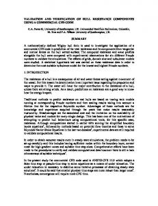
Fig. 5 Typical test stimulus. This image was obtained by applying an FEC level of 0.15 to the right side of the mirror image pair derived from the right side of the planes image.
has previously been used to model the appearance of images processed by a non-uniform visual system [ 181. Here we used the discrimination of wide-field imagery to test the validity of these previously-described simulations and to determine whether a single eccentricity-dependent parameter (i.e., the FEC) is sufficient to model the wellknown spatial non-uniformity of the visual system. We further attempted to determine which of several CSFs was the best estimator of the discrimination of complex, widefield imagery. 4.1
Methods
Six observers were tested, although not all under all experimental conditions. The observers ranged in age from 18 to 48 years, and had uncorrected 20/20 vision as determined by a Snellen chart. The observers were paid for their participation. Four stimulus images were obtained from the left and right halves of two digitized aerial photographs, one of airport buildings and the other of planes on the ground (Fig. 5). One half of each stimulus image was an unprocessed version of the original half-image, and the other was a mirror image of the original half-image (Fig. 5), processed as described below. The full stimulus images were 1024 x 1024 x 8-bits and subtended 64” at a viewing distance of 1.2 m. Stimuli were rear-projected onto a large screen (Lumiglas 130, Stewart Film Screen Corp.) using the green channel of a Barco Graphics 808s CRT. Stimulus presentation and data collection were controlled by an SGI Crimson workstation.
18-6
10
-
th gp extrapolated
2
l -
i
bc
.l
5 8 u .Ol
.OOl .Ol
.l
1
10
10
Frequency [cfdeg] Fig. 6. The three CSF data sets used in the various simulations. The gp (orientation defection/ variable window) set was obtained with Gabor stimuli in an orientation discrimination task. The th (pattern detection/ variable window) set was obtained using the same stimuli in a contrast detection task. The bc (pattern defection/ constant window) set was obtained with a fixed aperture grating stimuli in a detection task. Note that the bc and fh CSF are identical at midfrequencies of about 3 c/deg. Extrapolated values were used in the simulations when needed outside the available data range. To simulate their appearance across 64” of visual angle, the images were processed assuming fixation at their center. The details of the simulation method are given in Peli [8], and the modifications used for peripheral simulations are given in Peli et al. [ 181. The appropriate threshold at each location was determined using the fovea1 CSF data set and the FIX applied for a given simulation. The threshold was calculated for each eccentricity, 0, and for each FEC as: T(e, j) = T(0, f,
exp(FEC
. e.f>.
where T(O, fi is the fovea1 threshold frequency in cldeg.
(1) andfis
0.01
0.1
Fundamental Eccentricity Constant Fig. 7 Preliminary results repotted by Peli and Geri [16] and Peli [24]. The data fall on the active portion of the psychometric function, and the threshold FEC is close to the prediction. However, the percent correct is high even for very low levels of FEC (upper graph), and there is a significant image dependence (lower graph). Both effects are inconsistent with the present vision model. detection/constant window CSF data were based on contrast detection of sinusoid gratings within a 2” square aperture [23]. These data were band-pass in character and the absolute values for the mid-spatial frequency range were similar to that of the pattern detection/ variable window data (see Fig. 6). Whenever values outside the measurement range were needed for the simulations they were extrapolated as shown.
the spatial
The images were processed using one of three CSF data sets @attern detection/ constant window, orientation detection/variable window, or pattern detection/variable window) and one of seven FEC levels (0.02,0.035,0.055, 0.075,0.10,0.15, and 0.20). The FEC levels of 0.035 and 0.055 were found by Peli et al. [18] to fit various peripheral CSF data sets from the literature. The remaining FIX levels were selected to cover a suitable range around these values. The orientation detection/ variable window CSF data were based on the discrimination of horizontal and vertical l-octave Gabor patches (i.e., a sinusoid within a gaussian aperture) and were low-pass in character. The pattern detection/variable window CSF data were obtained using a contrast detection task and similar stimuli [ 151. These were also low-pass in character. The pattern
A total of 560 trials were run in each 1-hr. session. The 560 trials corresponded to 10 random presentations of each of 56 stimulus images (i.e., 4 original images x 2 sides for the standard x 7 FEC levels). The data presented here are means of five Percent-Correct estimates, each in turn obtained from the forty responses within an individual session. 4.2
Results
Preliminary results of this study, shown in Fig. 7, have been reported in part by Peli and Geri [ 161 and Peli [ 121. The smooth curves in the graphs represent the best-fitting, two-parameter Weibull function. The basic finding that the chosen FEC range resulted in a full psychometric function indicated to us that the simulations were approximately correct.
18-7
pattern detection I constant window orientation detection / variable window pattern detection / variable window Weibull fit
0
100
l A
90
I-
80 70 60 50 40
0.01
0.1
60
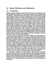
Fhmlamental Eccentricity Constant Fig. 8 Effect of the high-frequency residual on image dependence. Once the HFR (that was included in the images used for the results shown in Fig. 7) was removed, the image dependence was significantly reduced. A surprising result was that even for very low FEC values the discrimination of the simulation from the original was at a level much higher than the 50% chance. Such a result is possible since the images are processed by the fovea1 CSF even for an FEC of zero, and therefore they differ from the originals. However, it is important to note that for the low values used, the simulations were processed so little that they were difficult to distinguish when examined carefully side-by-side on the screen for unlimited time. Initially we suspected that the high level of discrimination in the periphery was a result of the abrupt short presentation [25]. However, changing the presentation waveform to a 500 msec gaussian did not change the results. Shown in Fig. 7 (lower) are means obtained from four observers for the two images used. The data indicate that the “planes” image simulation was easier to discriminate from the original than was the “city” image. Since the vision model is observer-based and includes no imagedependent parameters, it cannot account for this aspect of the data. We have seen similar effects in testing simulations of central vision [ 151, and in that case the effects were attributed to an artifact, the so-called high frequency residual (HFR), which was removed from the simulations but which remained in the original image. The HFR is the set of spatial frequencies at the comers of the square spatial-frequency support, which are excluded when only a circularly symmetrical filter is used. Peli [ 151found that removal of the HFR resulted in the elimination of the image dependency as well as an improved performance of his simulations at various viewing distances. The data shown in Fig. 8, again are means obtained from four observers, but were obtained using stimulus images from which the HFR had been removed. Although there is a small difference between the curves at one or two FEC levels, the image dependence has been significantly reduced. Shown in the upper graph of Fig. 9 are the functions relating the percent correct obtained in the discrimination task to FEC level for images simulated using either the pattern detection/constant window (open symbols) or orientation detection/variable window (closed symbols)
0.01
1 0.1
Fundamental Eccentricity Constant Fig. 9. A comparison of the discrimination data for images simulated using CSFs in turn obtained using various combinations of detection task (pattern or orientation) and stimulus window (constant or variable). The error bars are *l s.e.m. intervals about each data point. CSF functions. These data represent averages for four observers. The FEC level corresponding to 81.6 Percent Correct was 0.128 for the pattern detectiorJ constant window data and 0.091 for the orientation detection/ variable window data. Analogous data comparing the results for the pattern detection/ variable window and orientation detection/variable window CSF functions are shown in the lower graph of Fig. 9. The pattern detection/ variable window data were obtained for three of the four observers from whom the pattern detection/constant window and orientation detection/ variable window data were obtained. The average threshold IZC level for the pattern detection/variable window data was estimated to be 0.140. The results in Fig. 9 show a clear difference between the simulations based on the orientation detection and pattern detection CSFs, but cannot differentiate between the two data sets based on the constant window and variable window CSFs obtained using the pattern detection task. As shown in Fig. 6, the CSFs associated with these latter two data sets converge at middle frequencies. Since the constant window CSF show higher threshold than the variable window at low frequency, which are tested by low contrast images, we can expect the variable window simulations results to require higher FEC values to match. Thus, we can predict that the simulations would diverge and in a predictable manner if images of lower or higher
18-8
o 0
pattern detection / constant window pattern detection / variable window Weibull fit I
I
100
Contrast=O. 1
100
I
i
Contrast=0.3 0
90
90
80
‘&, j--------+!#
i
4
70
-ATi
60 50
,
40
80
40 j 0.01
I 0.1
I
I
1
--------
70 60 50 40
Fundamental Eccentricity Constant Fig. IO. The effects of image contrast error bars are *I s.e.m. intervals about
on the functions each data point.
contrast were used to test lower and higher frequencies, respectively. The one that would remain stable (if any) is the one representing the subjects’ perception. The experiments therefore were repeated using test images whose contrasts (actually amplitudes) were scaled by factors of 0.1,0.3, and 3.0 compared to the original image set. The results shown in Fig. 10 were indeed as expected. The results for the original image (contrast = 1 .O) essentially replicate, using a different set of observers, the previous data shown in Fig. 9. As the contrast was reduced, the I%C found for the constant-window condition remained largely unchanged (even though the slope of the psychometric function changed, especially for contrast = 0.1). For the variable-window condition, however, the FIX gradually increased as contrast was reduced. These results suggest that peripheral sensitivity decreases at lower spatial frequencies. This conclusion is consistent with the data of Fig. 10 obtained using images simulated with the constantwindow CSF (open circles), and is not consistent with the data obtained using images simulated with the variablewindow CSF (filled circles). In all cases, the FEC found in our experiments was higher than the 0.035 - 0.055 value we computed from a number of data sets published in the literature, where grating targets on a uniform background were used [18].
relating
Percent
Correct
discrimination
to FEC level. The
5. DISCUSSION The results of the foveal experiments verified that the model proposed by Peli [8] and used to simulate the appearance of an image from different observation distances is valid. The simulated images were found to be distinguishable from the original images at distances close to the simulated distances. Thus, these results demonstrate that the present simulation procedures can be used to determine whether the discrimination of complex images can be predicted from the form of empirically derived CSFs. Also of interest are the possible reasons for the differences between the CSF’s obtained here for different observation distances. Differences at the low frequency end are relatively easy to account for. The low frequency Gabor stimuli viewed from a distance of 2 m are quite large, and often extended to near the edge of the display area. The edge of the screen (outside the display areas) is dark and thus creates a high contrast feature which when close to the stimuli may reduce their visibility. Moving the observer closer to the screen reduces the size of the stimuli providing the same spatial frequencies, thus increasing their distance from the display edge and reduces its masking effect. Indeed for both observers the detection threshold for the three lowest spatial frequencies was almost equal at 2 m and 0.5 m (which were the same physical stimuli) suggesting that the low-frequency
18-9 reduction in sensitivity to these stimuli is, in fact, a masking effect. This argues for an even higher sensitivity at low frequencies than that represented by the “combined CSF” in Fig. 3. The reduction in high-frequency sensitivity that we found when observation distance was increased cannot be as easily explained.
image quality. In particular, the peripheral vision model suggested by the present analysis might be useful in evaluating wide field simulator images as well as area of interest, or other foveating systems.
The larger stimuli viewed at 4 or 8 m were closer to the edge, and hence may have been masked as the stimuli used to test the lower frequencies were assumed to be. These images were also of higher contrast, which might be hypothesized to result in more masking. However, such masking should reduce the sensitivity to these frequencies not improve it. Thus, at the moment we have no hypothesis that adequately explains this effect.
This work was supported in part by grants EY05957 and EY 10285 from the NIH, and by U.S. Air Force Contract F41624-97-D-5000 to Raytheon Training and Services Co. at the Air Force Research Laboratory, Mesa, Arizona. We thank Brian Sperry, Jack Nye, and Craig Vrana for programming support.
We found that by varying a single parameter (the FEC) in our simulation, we could vary discrimination gradually from chance level to 100%. This confirms the validity of the simulation technique and suggests that the FEC adequately represented the position-dependent changes in the appearance of our stimuli. The fact that wide-field images simulated using various fovea1 CSFs were discriminated at different FEC levels, extends to peripheral vision the findings of Peli [ 151, regarding the sensitivity of both the simulation and the psychophysical method to small differences in the CSF. The CSFs obtained with pattern detection tasks resulted in lower thresholds, thus it is not surprising that the simulations using the pattern detection/constant window and pattern detection/variable window CSFs led to higher FEC levels. The combination of lower fovea1 thresholds and higher FECs compensate for each other in computing peripheral thresholds. The foveal CSFs used in the simulations were complete functions of contrast sensitivity in that they differed in shape as well as absolute sensitivity. One may wonder how is it possible that such large differences in the form of the CSF can be compensated by changes in a single variable, the FEC, such that the threshold of discrimination remains the same. This is the case because, as pointed out by Peli [ 151 and confirmed by Peli [26], while the whole CSF is used in the generation of the simulation, only a very narrow range of frequencies (probably near the contrast sensitivity peak) is tested in the image discrimination task. The finding that the pattern detection/variable window CSF, which is very similar to the pattern detection/constant window CSF for midfrequencies (Fig. 6), resulted in similar threshold FE&, also further supports this conclusion. All FECs found here are larger than those computed from CSF measurements obtained across the retina (see Table 1 in Peli et al. [ 111). This difference may be due to masking by superimposed or adjacent image detail, which may result in a more rapid decline of detection performance as retinal eccentricity is increased (i.e., crowding or lateral masking effects). While such effects were demonstrated in a number of letter acuity tests, we are not aware of direct measurements of such lateral masking for gratings or grating patches. The vision model employed here produced images that were discriminable in a way predictable from wellestablished visual and perceptual data. It might, therefore, be expected that analogous models could be employed to assess more general image properties such as perceived
ACKNOWLEDGMENTS
REFERENCES 1.
Pelli, D., What is Low Vision? 1990, Institute for Sensory Research, Syracuse University: Syracuse, NY.
2.
Lundh, B.L., Derefeldt, G., Nyberg, S., and Lennerstrand, G., “Picture simulation of contrast sensitivity in organic and functional amblyopia”, Actu Ophthalmologica (Kbh), 59, pp. 774-783, 198 1.
3.
Ginsburg, A.P., Visual information processing based on spatialfilters constrained by biological data, in Aerospace Med. Res. Lab. Rep. 1978, Cambridge University: Wright-Patterson AFB, OH.
4.
Thibos, L.N. and Bradley, A., “The limits of performance in central and peripheral vision”, Digest of Technical Papers Society for Information Display, 22, pp. 301-303, 1991.
5.
Larimer, J., “Designing tomorrow’s displays”, Technical Briefs, 17(4), pp. 14-16, 1993.
6.
Lubin, J., “A visual discrimination model for imaging system design and evaluation”, in Vision Models for Target Detection, E. Peli, Ed. pp. 245-283, World Scientific, Singapore, 1995.
7.
Peli, E., Goldstein, R.B., Young, G.M., Trempe, CL., and Buzney, SM., “Image enhancement for the visually impaired: Simulations and experimental results”, Investigative Ophthalmology and Visual Science, 32, pp. 2337-2350, 1991.
8.
Peli, E., “Contrast in complex images”, Journal of the Optical Society of America [A], 7, pp. 2030-2040, 1990.
9.
Duval-Destin, M., “A spatio-temporal complete description of contrast”. in Digest of Technical Papers Society for Information Display, Society for Information Display, 1991.
NASA
10. Daly, S., “The visual differences predictor: An algorithm for the assessment of image fidelity”, Proceedings of the SPIE Vol. I666 Human Vision, Visual Processing, and Digital Display III,, pp. 2-15, 1992. 11. Peli, E., Yang, J., and Goldstein, R., “Image invariance with changes in size: The role of peripheral contrast thresholds”, Journal of the Optical Society of America [A], 8, pp. 1762-1774, 1991. 12. Peli, E., “Simulating normal and low vision”, in Visual Models for Target Detection and Recognition, E.Peli, Ed. pp. 63-87, World Scientific Publishers, Singapore, 1995.
18-10
13. Stephens, B.R. and Banks, M.S., “The development contrast constancy”, Journal of Experimental and Child Psychology, 40, pp. 528-547, 1985.
of
14. Brady, N. and Field, D.J., “What’s constant in contrast constancy? The effects of scaling on the perceived contrast of bandpass patterns”, Vision Research, 35(6), pp. 739-756, 1995. 15. Peli, E., “Test of a model of foveal vision by using simulations”, Journal of the Optical Society of AmericaA, 13, pp. 1131-1138, 1996. 16. Peli, E. and Geri, G., “Putting simulations of peripheral vision to the test”, Investigative Ophthalmology and Visual Science., 34 (4, suppl), pp. 820, 1993. 17. Schwartz, E.L., “Spatial mapping in the primate sensory projection: Analytic structure and relevance to perception”, Biology and Cybernetics., 25, pp. 18 l194,1977. 18. Peli, E., Yang, J., Goldstein, R., and Reeves, A., “Effect of luminance on suprathreshold contrast perception”, Journal of the Optical Society of America [A], 8, pp. 1352-1359, 1991. 19. Fiorentini, A.L., Maffei, L., and Sandini, G., “The role of high spatial frequencies in face perception”, Perception, 12, pp. 195-201, 1983. (esp. p. 196) 20.
Hayes, T., Morrone, M.C., and Burr, D.C., “Recognition of positive and negative bandpassfiltered images”, Perception, 15, pp. 595-602, 1986.
21.
Norman, J. and Ehrhch, S., “Spatial frequency filtering and target identification”, Vision Research, 27, pp. 87-96, 1987.
22. Parish, D.H. and Sperling, G., “Object spatial frequencies, retinal spatial frequencies, noise and the efficiency of letter discrimination”, Vision Research, 31, pp. 1399-1415, 1991. 23.
Cannon, M.W., Jr., “Perceived contrast in the fovea and periphery”, Journal of the Optical Society of America [A], 2, pp. 1760-1768, 1985.
24.
Peli, E., Visual Models for Target Detection and Recognition, Series on Information Display, Ed. H.L. Ong, Vol. 1. World Scientific Publishers, Singapore, 1995.
25.
Peli, E., Arend, L., Young, G., and Goldstein, R., “Contrast sensitivity to patch stimuli: Effects of spatial bandwidth and temporal presentation”, Spatial Vision, 7, pp. 1-14, 1993.
26.
Peli, E., “The contrast sensitivity function (CSF) and image discrimination”, in SPIE Proceedings Human Vision and Electronic. In press, 1999.