Validation Gating for Non-Linear Non-Gaussian Target Tracking Tim Bailey, Ben Upcroft and Hugh Durrant-Whyte Australian Centre for Field Robotics University of Sydney, NSW, Australia
[email protected] Abstract - This paper develops a general theory of validation gating for non-linear non-Gaussian models. Validation gates are used in target tracking to cull very unlikely measurement-to-track associations, before remaining association ambiguities are handled by a more comprehensive (and expensive) data association scheme. The essential property of a gate is to accept a high percentage of correct associations, thus maximising track accuracy, but provide a sufficiently tight bound to minimise the number of ambiguous associations. For linear Gaussian systems, the ellipsoidal validation gate is standard, and possesses the statistical property whereby a given threshold will accept a certain percentage of true associations. This property does not hold for non-linear non-Gaussian models. As a system departs from linear-Gaussian, the ellipsoid gate tends to reject a higher than expected proportion of correct associations and permit an excess of false ones. In this paper, the concept of the ellipsoidal gate is extended to permit correct statistics for the non-linear non-Gaussian case. The new gate is demonstrated by a bearing-only tracking example.
Keywords: Target tracking, data association, validation gating, Gaussian mixture models.
1
Introduction
Target tracking is the problem of estimating the location and velocity of one or more moving targets given a motion model and a set of sensor measurements [1]. Sensed data is imperfect and, moreover, a single measurement might detect only an aspect of a target position (e.g., range-only or bearing-only), so multiple measurements are combined using a stochastic filter. Sensor fusion involving non-distinct targets introduces the problem of data association. A measurement might originate from one of several targets or from clutter within the environment, and robust data association must deal with this ambiguity. A number of schemes exist in the literature including joint probabilistic data association (JPDA) [3], multihypothesis tracking (MHT) [10], and mixture model tracking (MMT) [7]. Each of these systems can be computationally prohibitive if all possible associations are considered, particularly when accounting for nondetection of existing tracks, false alarms, track loss, and new track detection. Furthermore, probabilities
of false positives (clutter) and false negatives (nondetection) are problem specific and may be difficult to model realistically. To reduce complexity for practical implementation validation gating is applied [1]. A validation gate is an association threshold, whereby an observation-to-target association is considered if it satisfies a metric of “acceptability”, and is rejected otherwise. Typically this gate is based solely on distance, although other attributes (e.g., colour, radar signature) might also act as discriminants. A data association scheme, such as MHT, becomes more tractable having first culled very unlikely associations. The standard validation gate is a Gaussian hyperellipsoid, and is an optimal metric for linear-Gaussian systems. It remains ubiquitous in the current target tracking literature [12, 8, 5, 11]. However, it ceases to be statistically precise for systems with non-Gaussian probability densities or non-linear observation models. As a system departs from linear-Gaussian, the ellipsoid gate tends to reject a higher than expected proportion of correct associations and permit an excess of false ones. This paper investigates validation gating for nonlinear non-Gaussian systems. It develops a general theory for validation gating as an extension to the linear concept of the ellipsoidal gate. For linear-Gaussian models, the new gate is identical to the ellipsoidal gate. For non-linear non-Gaussian models, it maintains a proper statistical “probability of acceptance” and continues to exhibit sensible gating behaviour. While this paper provides implementation of our theory, the focus is not on computational aspects but on theoretical concepts and intuitions of the key gating properties. The paper format is as follows. Section 2 defines the properties and calculation of the standard ellipsoidal gate. Section 3 presents a generic Monte Carlo solution for computing a validation threshold. Section 4 introduces the bearing-only scenario used as an example in subsequent sections. Section 5 presents a measure of validation likelihood based on the marginal observation density p (z), and examines why it is not sensible. The next section discusses why p (z) does, however, provide a proper measure of track likelihood. Section 7 presents a second measure of validation likelihood based on the joint target-measurement density p (x, z), and proposes that this is reasonable and general. The final section provides concluding remarks and suggestions for future research.
2
Ellipsoidal Validation Gate
3
The ellipsoidal validation gate is optimal for a linear observation model1 with additive noise z = Hx + r
(1)
where the state probability density function (PDF) is ˆ , P), and the noise is zeroGaussian p (x) = N (x; x mean Gaussian p (r) = N (r; 0, R) and independent of x. The validity of a measurement zi is determined from its residual (or innovation) with the predicted observation ν = zi − Hˆ x
(2)
which has covariance S = HPHT + R. Validation is computed by gating the normalised innovation squared (NIS).2 ν T S−1 ν < Md
(3)
The threshold Md , for an innovation dimension d, can be computed efficiently since the NIS follows a chisquare PDF. Thus, for a “probability that n% of true associations are accepted”,3 Md is obtained from n d Md = P( , ) 100 2 2 where 1 P (a, b) = Γ(a)
Z
b
e−t ta−1 dt
(4)
(5)
0
is the incomplete gamma function [9]. It is important to realise that a validation gate provides no statistical measure for the rejection of false associations. Rather, it defines a region of acceptance such that (100−n)% of true measurements are rejected given that each zi is distributed according to p (z) = N (z; Hˆ x, S)
(6)
This allows the gate to operate without recourse to models of clutter etc, which may be difficult to define realistically. Effectively, it eliminates very unlikely associations, the bulk of which are presumably other targets and clutter, and the remaining measurements, whether true or false, are plausible candidates. 1 It
is typical for state-space variables to have time-subscripts, such as xk , but, as validation gating is not time dependent, they are omitted here. 2 The NIS is also commonly known as the Mahalanobis distance. 3 This statement is a little misleading; the ellipsoidal gate as calculated from (4) does not accept a specified n% of true measurements in a real (physical) case. If the true target location xt is somewhere towards the centre of p (x), then more than n% of measurements, which are distributed according to p (z|x = xt ), will be accepted. If, on the other hand, xt is far from the mean of p (x), less than n% will be accepted. What the ellipsoidal gate does achieve is the acceptance of n% of true measurements over a series of Monte Carlo simulations, where xt is sampled from p (x) for each run. This statistical quality is the same for the non-linear validation gates developed in this paper.
Computing a Validation Gate for Non-Gaussian PDFs
A closed-form validation threshold is not, in general, available for non-Gaussian PDFs. However, an approximation is possible via Monte Carlo sampling. 1. Draw N samples zi ∼ p (z). 2. Weight each zi according to its likelihood of “association validity”. 3. Select the m-th largest weight, where m = N n/100, to obtain an n% acceptance threshold, wn . Thus, if n is large (say 95%), then wn is small, (the bottom 5%). If the validation likelihood of a particular measurement is greater than wn , then the association is accepted. For p (z) Gaussian, this approach becomes equivalent to the ellipsoidal gate as N → ∞. From the above algorithm, steps 1 and 3 are straightforward. Samples drawn from p (z) provide a statistic of how many measurements will fall within a certain region of observation-space, and selecting an ordered weight marks a bound for inside or outside that region. Step 2, on the other hand is less intuitive, and the remainder of this paper focuses on defining an appropriate measure for validation likelihood. Two measures are investigated. The first is the observation PDF p (z), such that wi = p (z = zi ). This measure, while seemingly the obvious solution, is shown to be an unreasonable validation likelihood. The second is based on the joint PDF of the state and observation p (x, z). Given an observation zi , the validation likelihood is wi = max p (x, z = zi ); the mode of a slice along zi . This measure gives sensible gating results. Both measures are equivalent to the standard ellipsoidal gate for linear-Gaussian systems.
4
Bearing-Only Tracking
As an example of a non-linear non-Gaussian problem, we consider a bearing-only target tracking scenario. The bearing observation model is given by µ ¶ y − ys z = h (x, xs ) + r = arctan +r (7) x − xs where r is zero-mean Gaussian with variance R = (π/360)2 , and the sensor location xs is assumed perfectly known. For a given target location xi , this model defines the conditional PDF p (z|x = xi ) = N (z; h (xi , xs ), R) and, for a given measurement zi , it defines the likelihood function p (z = zi |x) over the domain of x. A bearing-only likelihood function p (z = 0◦ |x), in the Cartesian plane, is shown in Figure 1. Note, this function differs from the model in (7) in two respects. First, it is a Gaussian mixture model (GMM) approximation, which permits relatively efficient computation. And second, due to the limited number of mixture components, it exhibits a roll-off in likelihood after about
10 8 6 4 metres
2 0 −2 −4 −6 −8 −10
0
50
100
150
200 metres
250
300
350
400
(a) Gaussian components (2σ ellipses) and 95% volume bound
(b) GMM likelihood function
Figure 1: A 20-component Gaussian mixture model of a bearing-only likelihood function in the coordinate frame of the target x, where xs = [0, 0]T and z = 0◦ . The individual components are shown in (a), along with an equi-likelihood contour encompassing 95% of the GMM probability mass. 300 metres, whereas (7) defines a constant likelihood along the x-axis from the origin to infinity. Likelihood functions for other bearing angles, taken from different sensor locations, have the same essential shape as in Figure 1, just shifted and rotated to the appropriate position and angle. Given an uninformative prior, say p (x) = N (x; 0, ∞), Bayesian fusion with p (z = zi |x) produces a posterior p (x|zi ) with the same shape as the likelihood function, but normalised to unit volume. In the remainder of this paper, we use p (x|z = 0◦ ) as the prior PDF in our examples; that is, the fusion of the likelihood function in Figure 1 with an uninformative prior over the domain of x. For notational convenience, we denote this (informative) prior as simply p (x). It is the PDF of the target location based on a single bearing-only measurement. The bearing-only scenario is interesting because the observation model is very non-linear. In particular, p (x) has a region of high probability density but little local probability mass near the origin; the bulk of the mass is distant from the origin. This is different to a Gaussian PDF, where the region of most mass is also the region of high likelihood. The existence of high likelihood away from the concentration of mass is fundamental to the derivation of a suitable gating measure.
Thus, a particular zi is accepted if p (z = zi ) > wn . In general, p (z) can be obtained from the observation model and the prior as Z p (z) = p (z|x) p (x) dx (9) which is a marginalisation over x of the joint PDF p (z, x). If the observation model is linear, as in (1), and the PDFs are represented by GMMs, p (x) =
N X
ˆ i , Pi ) αi N (x; x
(10)
βj N (r; ˆrj , Rj )
(11)
i=1
p (r) =
M X j=1
then there is a closed-form solution. p (z) =
N X M X i
αi βj N (z; Hˆ xi + ˆrj , HPi HT + Rj )
j
(12) However, for a non-linear observation model an approximation is required. In our experiments, we chose a simple, though expensive, Monte Carlo sampling approach. 1. Draw N samples xi ∼ p (x). 2. The conditional PDF is p (z|xi ) = h (xi ) + p (r).
5
p(z) as a Validation Likelihood
The generic gating algorithm in Section 3 draws samples from p (z), and so the most intuitive measure of validation likelihood is p (z) itself. Certainly for the Gaussian case in (6), an n% acceptance threshold based on p (z) is equivalent to the standard chi-square gate, and can be computed directly as ¶ µ 1 exp − Md wn = p 2 (2π)d |S| 1
(8)
conditionals to marginalise over x, 3. Sum the P N p (z) ≈ N1 i (h (xi ) + p (r)). For the model in (7), with p (r) Gaussian, we get N 1 X p (z) ≈ N (z; h (xi , xs ), R) N i
(13)
Figure 2 shows an example validation gate obtained for the prior p (x) from Section 4 when the sensor location is moved to xs = [10, 10]T . The resulting p (z)
20
p(z)
15
10
5
0 −40
−35
−30
−25
−20 −15 z (degrees)
−10
−5
0
5
(a) p (z)
(b) Gate on p (z)
Figure 2: Validation gate for a bearing-only scenario, where p (x) is depicted in (b) by a shaded green region (marking 95% of its mass), and the sensor location xs = [10, 10]T by a ∗. The threshold weight w95 is shown by a horizontal line in (a), and the resulting region of valid bearing observations radiating from xs are shown in (b) by the shaded blue region.
Clearly, rejecting angles less than -10◦ , means rejecting observations that, intuitively, are quite feasible; effectively it rejects the possibility of a target close to the origin. For example, from p (x), the probability density of the true target location being at, say, [50, 0]T is equal to it being at [250, 0]T . This agrees with our intuition where, based on a single bearingonly measurement, we would not be surprised if the target turned out to be near the origin. However, if the true target was at xt = [50, 0]T , so that observations actually received are distributed according to p (z|x = xt ), 95% of observations would fall between -15◦ and -13◦ , and all of them would be rejected by this validation gate. The problem with p (z = zi ) is that its meaning— “the likelihood of obtaining zi when xt could be anywhere in p (x)”—does not correspond to our essential requirement for a validation gate. From p (z) we predict an observation is most likely to come from the direction where concentration of mass in p (x) is greatest; this is apparent from Figure 2(a). However, the likelihood of an observation is not the same as the feasibility of an observation. From the density of p (x) it is clear that a target location at [50, 0]T is as feasible as at [250, 0]T . Thus, we make the following distinction. Before any measurement has been received, the density of p (z) predicts which observations are most likely, while, having received a particular observation zi , the density of p (x) indicates whether it might originate from a feasible target. We contend that a validation gate is concerned with the feasibility of an existing measurement, not the likelihood of a measurement yet to arrive. 4 For
clarity, the coordinate axes in Figure 2(b), and subsequent figures, are not equal. However, this has the unfortunate effect of exaggerating angles, which distorts the true shape of the validation region, making it appear much larger than it really is.
10 8 6 4 metres
is shown in Figure 2(a). Sampling from p (z), 95% of samples lie between -10◦ and -0.36◦ , and the threshold weight w95 is 0.5. Thus, observed angles must be -10◦ < zi < -0.36◦ to be accepted; this is depicted in Figure 2(b).4
2 0 −2 −4 −6 −8
0
50
100
150
200 metres
250
300
350
400
Figure 3: A multiple hypothesis example, where p (x) and xs are as in Figure 2. The sensor returns two measurements, shown as lines, at −10◦ and −2◦ . The two possible updates for the target are depicted by contours bounding the 95% mass concentration of the respective posterior PDFs.
6
p(z) as a Measure of Track Likelihood
While not sensible as a measure of validation, p (z) is a reasonable measure of track likelihood when there exist multiple track hypotheses. Consider the example in Figure 3. The prior p (x) and sensor location xs are the same as in Figure 2, and it is known that there exists a single target only. However, the sensor returns two measurements, z1 = −10◦ and z2 = −2◦ , one of the target and the other of clutter. If the clutter is assumed to be uniformly distributed, then there are two possible hypotheses: H1 :
z1 = h (x, xs ) + r 1 , −π < c ≤ π 2π 1 , −π < c ≤ π z1 = c, p (c) = 2π z2 = h (x, xs ) + r z2 = c,
H2 :
p (c) =
(14)
(15)
These hypotheses may be ranked, as to one being more likely than the other, by a general mechanism known as Bayesian model comparison [6, Chapter 28]. Whenever performing an update using Bayes theorem,
the models of the system are always an implicit conditioning parameter H. p (x|z, H) =
p (z|x, H) p (x|H) p (z|H)
(16)
Typically, the posterior is computed as proportional to the numerator of the right-hand-side, and p (z|H) is ignored as a normalising constant. When there exist multiple alternative hypotheses {H1 , . . . , HN }, however, the value of p (z = zi |Hm ) is the “evidence for Hm ”; it quantifies the relative merit of a hypothesis for predicting the observation zi , and allows different models to be ranked. In our example, where z = [z1 , z2 ]T is the pair of observations, p (z|H) = p (z1 |H) p (z2 |H) as z1 and z2 are independent. Given the measurement z1 = −10◦ and the hypothesis H1 , the scalar value of p (z1 |H1 ) is computed as Z p (z1 |H1 ) = p (z1 |x, H1 ) p (x) dx (17)
through the joint PDF p (x, z = zi ) along the hyperplane z = zi .5 The value of p (x, z = zi ) at each point xj is the probability that both zi is valid and the true target location is xj . The mode xmode = arg max p (x, z = zi )
(21)
gives the most likely target location possible for zi . We propose that the mode-weight of p (x, z = zi ) is the correct measure for likelihood of “association validity” for zi . Restating the algorithm from Section 3, the full validation gate computation is performed as follows. 1. Draw N samples zi ∼ p (z). Note, it is not necessary to compute p (z) in order to draw samples from it. Samples may be generated as xi ∼ p (x) then zi ∼ p (z|xi ). 2. Weight each zi according to its validation likelihood. (a) Generate the likelihood function p (z = zi |x).
For a GMM implementation, the prior and likelihood function are each weighted sums of Gaussians over the domain of x. p (x) =
N X
ˆ i , Pi ) αi N (x; p
(18)
i
p (z1 |x, H1 ) =
M X
ˆ j , Qj ) βj N (x; q
(19)
j
Therefore, the value of (17) is found by multiplying (18) and (19) and summing the weights of the resultant GMM. This integral can be computed directly as p (z1 |H1 ) =
N X M X i
j
αi βj
2π
1 p
µ ¶ 1 exp − ν T S−1 ν 2 |S| (20)
where ˆi − q ˆj ν=p S = Pi + Q j Computing p (z2 |H2 ) is similar. The value of p (z2 |H1 ) and p (z1 |H2 ) is simply 1/2π. This gives the ranking weights as p (z|H1 ) = 0.06 and p (z|H2 ) = 2.8. Thus, the hypothesis that z2 observes the target is by far the more likely model. This result makes sense as p (z) predicts that targets more distant from the origin are more likely, therefore the hypothesis supporting the more distant target has higher probability.
7
p(x,z) as a Validation Likelihood
Another possible measure of validation likelihood is the joint PDF p (x, z) = p (z|x) p (x). Given an observation zi , the product of the likelihood function p (z = zi |x) and the prior p (x) produces a slice
(b) Compute a slice of the joint PDF along zi , p (x, z = zi ) = p (z = zi |x) p (x). (c) Compute the mode wi = max p (x, z = zi ). 3. Select the m-th largest weight, where m = N n/100, to obtain an n% acceptance threshold, wn . Step 2(b) is the product of the likelihood function and the prior; this operation has a closed-form for both Gaussians and GMMs. Step 2(c) is closed-form for Gaussians, since the mean of p (x, z = zi ) is also its mode, but there is no analytical solution for GMMs. To find the mode of a general GMM requires a global optimisation algorithm. We implemented the search using a combination of Monte Carlo sampling and local optimisation, but more efficient solutions exist (e.g., [2]). When p (x, z = zi ) is Gaussian, its mode is proportional to its volume, i.e., max p (x, z = zi ) ∝ p (z = zi ) for all zi . Therefore, for linear-Gaussian models, the p (x, z) gate is equivalent to the p (z) gate and, in turn, to the standard ellipsoidal gate. Returning to the bearing-only example from Section 5. The samples drawn from p (z) are the same as before, but are weighted according to the mode of p (x, z = zi ), as shown in Figure 4(a). (Note, the top of Figure 4(a) should be flat, but a ripple is introduced by the GMM approximation.) Because the samples are from p (z), the resultant weight threshold w95 = 0.013 accepts 95% of true measurements, the same as for the gate in Section 5. But this time, the 5% rejected are those that intersect with p (x) along regions of low joint probability. In Figure 4(b) the valid region −135◦ < zi ≤ −1◦ includes locations close to the origin, as is expected intuitively. A point on the joint PDF p (x = xj , z = zi ) is the probability of xj and zi both being true together. 5 Be careful to avoid confusion here. A slice through the joint p (x, z = zi ) is not the same as the conditional p (x|z = zi ).
0.04 0.035
max p(x,z=z0)
0.03 0.025 0.02 0.015 0.01 0.005 0 −150
−100
−50
0
z (degrees)
(a) Mode of p (x, z = zi )
(b) Gate on max p (x, z = zi )
Figure 4: The values of p (x) and xs in (b) are the same as in Figure 2(b). In (a), the mode of p (x, z = zi ) is shown as a function of zi . The weighted samples from p (z) are red crosses, and the threshold weight w95 is shown by a horizontal line. The valid observation region is shown in (b) by the shaded blue region. Given a measurement zi , the mode of p (x, z = zi ) indicates the most likely target location possible for zi . If zi permits a likely target location, it is considered to be feasible, and so p (x, z = zi ) seems a reasonable measure for a validation gate.
8
Conclusion
This paper extends the concept of the ellipsoidal validation gate to non-linear non-Gaussian systems. The proposed gate is based on the joint target-observation PDF p (x, z) and exhibits the same “probability of acceptance” characteristics as the ellipsoidal gate. An alternative gate, based on the marginal observation PDF p (z), was found to be unsuitable. It tends to reject observations which intuitively seem possible and, indeed, would be probable if the true target location happens to be in a region of high probability density but low mass concentration. The problem is that p (z) is a predictive measure for the likelihood of future observations, whereas validation requires a feasibility measure for an observation actually received. Nevertheless, p (z) is a legitimate Bayesian measure of track likelihood when tracking multiple target hypotheses. The algorithms in this paper are computationally intensive, and our focus has been on theoretical aspects rather than actual implementation. We expect that more efficient approximations will be found (e.g., applying the unscented transform [4] to non-linear GMM transformations rather than Monte Carlo sampling). The main contribution of this paper is to develop a theory concerning the form of an ideal validation gate. We propose that the mode of p (x, z = zi ) is the correct measure, giving the right acceptance statistics and permitting feasible associations. As a fundamental measure, it provides a yardstick for comparing the veracity of heuristic or approximate gates developed for practical application.
Acknowledgement This work is supported by the ARC Centre of Excellence programme, funded by the Australian Research Council (ARC) and the New South Wales State Government.
References [1] Y. Bar-Shalom and T.E. Fortmann. Tracking and Data Association. Academic Press, 1988. [2] M.A. Carreira-Perpi˜ na ´n. Mode-finding for mixtures of Gaussian distributions. IEEE Transactions on Pattern Analysis and Machine Intelligence, 22(11):1318–1323, 2000. [3] T.E. Fortmann, Y. Bar-Shalom, and M. Scheffe. Sonar tracking of multiple targets using joint probabilistic data association. IEEE Journal of Oceanic Engineering, 8(3):173–184, 1983. [4] S. Julier, J. Uhlmann, and H.F. Durrant-Whyte. A new method for the nonlinear transformation of means and covariances in filters and estimators. IEEE Transactions on Automatic Control, 45(3):477–482, 2000. [5] T. Kirubarajan and Y. Bar-Shalom. Probabilistic data association techniques for target tracking in clutter. Proceedings of the IEEE, 92(3):536–557, 2004. [6] D.J.C. MacKay. Information Theory, Inference, and Learning Algorithms. Cambridge University Press, 2003. [7] L. Pao. Multisensor multitarget mixture reduction algorithms for tracking. Journal of Guidance, Control, and Dynamics, 17(6):1205–1211, 1994. [8] L.Y. Pao and R.M. Powers. A comparison of several different approaches for target tracking with clutter. In American Control Conference, pages 3919–3924, 2003. [9] W.H. Press, S.A. Teukolsky, W.T. Vetterling, and B.P. Flannery. Numerical Recipes in C. Cambridge University Press, 2nd edition, 1992. [10] D.B. Reid. An algorithm for tracking multiple targets. IEEE Transactions on Automatic Control, 24(6):843– 854, 1979. [11] J. Vermaak, S.J. Godsill, and P. P´erez. Monte Carlo filtering for multi-target tracking and data association. IEEE Transactions on Aerospace and Electronic Systems, 41(1):309–332, 2005. [12] X. Wang, S. Challa, and R. Evans. Gating techniques for maneuvering target tracking in clutter. IEEE Transactions on Aerospace and Electronic Systems, 38(3):1087–1097, 2002.