of the computed tip vortices and also a small improvement in the blade .... equations were discretisted using the second order finite volume method. (Jasak, 1996) and ..... no definitive conclusions can be drawn at this stage near the root of.
Validation of an Actuator Line Method for Tidal Turbine Rotors Aidan Wimshurst, Richard Willden Department of Engineering Science, University of Oxford, Oxford, United Kingdom
ABSTRACT Computations of the blade loading and the local flow field around the Model Rotor Experiments In Controlled Conditions (MEXICO) rotor are presented using an actuator line method, implemented within the open source code OpenFOAM. The nacelle and near wake mesh refinement are shown to have little influence on the computed blade loads but a significant impact on the near wake flow field. In addition, the blade loads and near wake flow field calculated with 3 different distributions of the Gaussian smearing parameter � are compared with experimental measurements. Local chord and lift coefficient scaled smearing distributions are shown to yield a significant improvement in the representation of the computed tip vortices and also a small improvement in the blade loading prediction, when compared with a spanwise constant smearing distribution. Despite these improvements in performance prediction, the performance of the rotor is shown to be more strongly influenced by the tip correction factor, where considerable improvement is still required before actuator line methods can represent real rotors with sufficient accuracy.
KEY WORDS: Actuator Line Method; MEXICO; OpenFOAM; Rotor Aerodynamics; Blade Loading; Tip Vortices.
INTRODUCTION The actuator line method (Sørenson and Shen, 2002) is particularly appealing as a computationally efficient technique for the representation of wind and tidal rotors. Viscous effects are captured through 2D aerodynamic data as a sub grid model, thus avoiding the necessity of resolving the rotor blade boundary layers. This 2D data is then used to build a virtual representation of the rotor blades, which are then rotated through a fixed grid to simulate the interaction of the rotor with the flow. The sub-grid blade model is both kinematically and dynamically coupled to the flow field calculation. However, the accuracy of the actuator line method in representing real rotors remains uncertain, in particular due to 3D flow effects that are not represented in the original 2D aerodynamic data. In this study, a comparison is made of the calculated blade loads and resulting flow field between the actuator line method and the Model Rotor Experiments In Controlled Conditions (MEXICO) rotor, with the aim of assessing the accuracy of the actuator line method for future wind and tidal rotor computations. Particular focus is placed on the mesh
sensitivity, Gaussian load smearing and tip correction factors that are often applied in actuator line computations. The MEXICO rotor is a 3 bladed horizontal axis 4.5m diameter rotor that was placed in the 9.5m × 9.5m open section of the Large Low-speed facility (LLF) of the German-Dutch Wind Tunnels (DNW) in 2006. Subsequent analysis of the experimental data from the MEXICO experiments took place under IEA Wind Task 29 Mexnext as an international collaborative project. The first phase of this project ended in 2011 with several aerodynamic codes validated and the source of many uncertainties highlighted (Schepers et al. 2012). In the MEXICO experiments, the rotor was operated at rotational speeds of 324.5 rpm and 424.5 rpm and at yaw angles between +30◦ and −30◦ for tunnel speeds of 10 m/s, 15 m/s and 24 m/s. These tunnel speeds were chosen to achieve a turbulent wake state, design condition and post-stall conditions for the rotor. In this report, only the results for the design condition (a tunnel velocity of 15 m/s, a rotational speed of 424.5 rpm, tip speed ratio of 6.67 and zero yaw, at a blade pitch angle of -2.3◦ ) will be presented. Like the NREL Phase VI rotor experiments, the MEXICO rotor was highly instrumented. Measurements of the blade pressure distribution were taken at 25%, 35%, 60%, 82% and 92% of the blade span, with a total of 148 Kulite pressure sensors distributed between these spanwise stations. At a rotational speed of 424.5 rpm, stereo particle image velocimetry (PIV) measurements were also taken in the vicinity of the rotor plane to complement the measured blade loading. The location of the radial PIV traverses considered in this work are shown in Fig. 1, along with the coordinate system adopted. These PIV measurements represented a considerable addition over previous experimental data sets such as the NREL phase VI experiments and was the primary reason for selecting the MEXICO rotor dataset to validate the actuator line method.
NUMERICAL METHOD In the MEXICO experiments compressibility effects were found to be negligible (Schepers et al. 2012) and hence in this investigation the incompressible Reynolds Averaged Navier-Stokes (RANS) equations were solved for the mean flow variables. To achieve closure of the RANS equations, the kinematic eddy viscosity νt was calculated using
θ = 0°!
where xi is the location of the collocation point on the ith blade, r is the spanwise distance along the blade, R is the rotor radius, ζ is the distance between the collocation point and the point in the fluid domain and � is the Gaussian width parameter. The influence of the Gaussian width parameter on the performance prediction for the MEXICO rotor will be considered in more detail later on.
PIV Traverse θ
z! y!
As explained by Shen et al. (2005) the concept of a correction factor was originally introduced into blade element momentum (BEM) models as a correction to the axial induction factor at the disc plane, to account for the finite number of blades on a real rotor or propeller. In the actuator line method, the rotor representation already has a finite number of blades. However a correction is still required. This is because at the blade tip, the pressure must equalise between the pressure and suction surfaces and hence the blade force must tend to zero. With no correction, blade element theory predicts a non zero force at the tip, unless the relative velocity is zero. Therefore a correction is still required for the actuator line method to ensure that the blade force tends to zero, regardless of the relative velocity at the blade tip. In this investigation, the 2D aerodynamic coefficients (C L and C D ) were multiplied by the tip correction factor F1 developed by Shen et al. (2005),
x
r!
r = R!
!
y = 2.75m
y = 1.18m!
Fig. 1 Schematic diagram of the coordinate system adopted, showing the location of the radial PIV traverse and the rotor azimuthal position θ measured clockwise from top dead centre. The streamwise flow direction is into the page.
the two equation k − ω SST turbulence model originally proposed by Menter (1994) but with the updated model coefficients of Menter et al. (2004). The body force applied by the rotating actuator lines was added as an additional source term S to the right hand side of the RANS equations, following Sørenson and Shen (2002). In the actuator line method, each rotor blade is discretised using a blade element approach into several spanwise segments. In this investigation a cosine distribution of segments was adopted, in order to increase the density of these segments towards the blade root and tip. During each iteration, the velocity at the location of each of these segments is returned from the flow solver. In this investigation the potential flow equivalence technique of Schluntz and Willden (2015) was used to determine the angle of attack α and velocity Urel relative to the local chord, at each blade segment. Following convention, these quantities were evaluated at the blade quarter chord (the collocation point). Using blade element theory, 2D lift and drag polars are then interpolated to determine the lift and drag coefficients (C L and C D ) at each collocation point, from which the total lift and drag forces can be readily calculated. The original aerodynamic data provided as part of the Mexnext project (Boorsma and Schepers 2009) was adopted, to allow direct comparison with other published work. The total blade force (given by the vector addition of the lift and drag forces) was then applied to the fluid domain as a source term S by numerically smearing the local blade force F across several cells, to mitigate numerical instabilities. Following Sørenson and Shen (2002) a Gaussian regularisation kernel η was adopted for the smearing,
S(x) =
N Z X i=0
R
F(r)η(|x − xi |)dr
(1)
0
" 2# −ζ 1 η(ζ) = 3 3/2 exp 2 � π �
(2)
!# " 2 N(R − r) −1 F1 = cos exp −g1 π 2r sin (φ)
(3)
g1 = exp (−c1 (Nλ − c2 )) + 0.1
(4)
where N represents the number of blades and φ the relative flow angle. The constants c1 = 0.125 and c2 = 21.0 were originally determined by curve fitting to experimental data from the NREL Phase VI rotor at a low tip speed ratio (λ = 3.79) and the Swedish WG 500 rotor at a high tip speed ratio (λ = 14.0). Due to the specific calibration of the empirical function with experimental data, its performance prediction was expected to be limited when applied to the MEXICO rotor under consideration here. The governing equations were solved using the open source code OpenFOAM (version 2.3.1) with the actuator line method implemented as an additional shared object library, developed at the University of Oxford. OpenFOAM adopts a collocated, cell centred approach for all flow variables with a Rhie and Chow (1983) type face interpolation procedure to prevent odd/even pressure decoupling. The governing equations were discretisted using the second order finite volume method (Jasak, 1996) and solved in terms of pressure-velocity variables in a Cartesian coordinate system. In this investigation the PISO algorithm of Issa (1984) was adopted for pressure-velocity coupling, with two pressure corrector loops each time step. Central differencing was applied for face interpolation of the Laplacian and gradient terms, second order implicit backwards differencing was applied for the temporal derivative (Jasak, 1996) and the flux limited form of central differencing using the Sweby (1984) flux limiter was applied for the convection terms. For consistency with Shen et al. (2012) a fixed time step ∆t = 10−3 R/U∞ was adopted for the computations. Temporal convergence was deemed to have occurred once the integrated rotor thrust and torque were within 0.1% of their final values. Increasing the number of pressure corrector loops to improve the convergence within each time step led to negligible change in the computed blade loads. Therefore the RANS equations were also deemed sufficiently converged within each time step.
implementation of the actuator line method to represent the rotor blades. A simplified representation of the tower was therefore not included in the computational domain. The turbulence intensity in the German-Dutch LLF was estimated to be less than 0.4% (Schepers et al. 2012). Therefore for this investigation uniform profiles of turbulent scalars k and ω were applied at the domain inlet, corresponding to a turbulence intensity of 0.4% and a representative length scale of 0.1cavg (where cavg is the average blade chord). On the domain lateral boundaries, zero gradient boundary conditions were applied for all mean flow variables. At the domain outlet, zero gradient boundary conditions were applied for all mean flow variables, except for pressure which was assigned a fixed value of 0. For the upstream boundary, a uniform fixed value of 15 m/s was applied.
GEOMTERIC CONSIDERATIONS
Fig. 2 Cut through a quarter section of the block structured mesh at the rotor plane (x = 0).
COMPUTATIONAL DOMAIN The MEXICO rotor was placed in the open section of the DNW making the blockage provided by the rotor difficult to precisely define. Previous calculations reported by Schepers et al. (2012) estimated the effective blockage of the model to be less than 1%. In addition Shen et al. (2012) made a comparison of the flow past the MEXICO rotor in unblocked conditions (a blockage ratio less than 1%) and with the tunnel geometry explicitly included. They concluded that blockage effects were insignificant, with a maximum increase in axial velocity of 3% at the rotor plane for the high tip speed ratio case. Therefore in this investigation, an unblocked configuration was adopted in order to avoid the computational complexity and expense of resolving the entire tunnel geometry. Specifically, a domain width and height of 10D were chosen to achieve a rotor blockage ratio of π/400 = 0.79%. The domain inlet was then placed 2.5D upstream of the rotor plane and the domain outlet 7D downstream of the rotor plane. A block structured mesh was adopted around a simplified form of the nacelle, with a polar layout to achieve axial symmetry over the swept area of the rotor. A cut through the block structured mesh at the rotor plane to demonstrate the polar layout, is shown in Fig. 2. The cell centroids adjacent to the nacelle were placed at a distance of 2.5 × 10⁻³ m normal to the wall, with a subsequent growth ratio of 1.1 away from the wall. This cell size was chosen such that the wall adjacent cell centroids were placed everywhere within the logarithmic law region of the universal law of the wall (Pope 2000). This wall normal distance allowed the velocity profile between the wall adjacent cell centroid and the wall to be modelled using the standard logarithmic law velocity profile (Pope, 2000). As shown later, the influence of the nacelle on the blade loading and resulting flow field was not of primary concern in predicting the performance of the rotor. Therefore the errors associated with inaccurate representation of the near wall flow (specifically the unsteady separation process) from the logarithmic law velocity profile assumption and simplified nacelle representation were not considered important for this investigation. Furthermore once per revolution loading from the tower shadow was not of interest for validating the
The nacelle geometry is often neglected in actuator line computations to avoid resolving the nacelle boundary layer and unsteady separation process. As a result, a central jet of fluid is allowed to pass through the rotor and the flow approaching the rotor is no longer deflected by the nose cone. Before proceeding with further investigations, the influence of the nacelle on the blade loading was briefly examined. Fig. 3 shows the axial and tangential blade loads per unit span computed with and without the simplified nacelle, using the original aerodynamic data (OAD) from Boorsma and Schepers (2012). Note that in this investigation, the axial and tangential forces refer to the forces normal and tangential to the blade in the global coordinate system (following Shen et al. (2012)) rather than in a local coordinate system aligned with the local chord at each spanwise section (following Plaza et al. (2015)). The actuator line computations of Shen et al. (2012) are also shown for comparison and in general show excellent agreement with the OpenFOAM computations. Overall for cases with and without the simplified nacelle, little difference was observed in the spanwise blade loading, with the greatest difference occurring in the tangential force near the blade root. Hence, the integrated rotor thrust and torque only showed an increase of 0.07% and 0.05% respectively with the removal of the nacelle. The sharp jump in axial and tangential forces along the mid-span of the blade has been attributed to the inconsistency between the RISØ-A1-21 aerodynamic data and the neighbouring DU91-W2-250 and NACA64-418 aerofoils used in the experiments, although there was a transition piece in between these (Shen et al. 2012). To alleviate this issue Shen et al. (2012) modified the aerodynamic data (MAD) to ensure a smoother transition between the aerofoils. Calculations with the aerodynamic data modified according to Shen et al. (2012) are also shown in Fig. 3. When adopting the modified aerodynamic data, the sharp transition was mostly removed and better agreement was found with the experimental measurements. However, this was not deemed a sufficient criteria to adopt the modified aerodynamic data for the remaining computations presented here. Fig. 4 compares the axial velocity U x along a radial traverse that coincides with the experimental radial PIV traverse for a rotor azimuthal position of 0◦ . The original aerodynamic data (with and without the nacelle) showed better agreement with the experimental measurements along the mid span of the blade, whereas the modified aerodynamic data showed a relatively poor agreement. This is because the modified aerodynamic data adopted a smoother transition between the aerofoil lift and drag polars. Therefore the change in bound circulation along the mid span of the blade was reduced, so less vorticity was shed into the wake. As a result, the axial velocity did not follow the experimental data
Fig. 4 Instantaneous axial velocity profiles U x extracted along a radial traverses 0.3m downstream of the rotor on the horizontal plane z = 0, for a rotor azimuth θ = 0◦ , comparing the influence of the nacelle representation and modified aerodynamic data.
tidal farm modelling. The importance of the nacelle geometry should therefore ideally be assessed in relation to the purpose of the simulation.
MESH SENSITIVITY
Fig. 3 Blade forces per unit span for the design tip speed ratio (U∞ = 15 m/s, λ = 6.67) comparing the influence of the nacelle representation and modified aerodynamic data.
well along the mid span of the blade. Hence, due to the lack of rigorous justification for the modification of the aerodynamic data and the poor resulting flow field representation, the original aerodynamic data was adopted for the remainder of the computations. While the effect of the nacelle on the blade loading was relatively small, the change in the resulting flow field was more appreciable and is visible in Fig. 4. To satisfy continuity, the axial velocity was increased along the entire radial traverse when the nacelle was included, with a maximum difference of 0.26 m/s at y = 0.66m (excluding the near wall flow). In general the axial velocity along the blade span showed excellent agreement with and without the nacelle included and the increase in axial velocity from the presence of the nacelle reduced towards the blade tips. It therefore appeared that the blade loading and near wake flow field could be reasonably well represented without the nacelle included explicitly in the computational domain. However the central fluid jet was still expected to influence the far wake mixing and therefore the overall wake recovery, which may be of importance for wind and
The initial mesh was generated with a similar level of refinement to that of Shen et al. (2012). In the axial (x) direction, 120 cells (N x ) with a constant edge length (∆ x ) of R/30 = 0.075m were assigned to the vicinity of the rotor (−0.5D < x < 1.5D). Upstream and downstream of this region, cells were allowed to expand in the axial direction with a growth ratio of 1.2. In the azimuthal (θ) direction, 198 cells (Nθ ) were evenly spaced around the circumference of the polar mesh structure to achieve an edge length (∆θ ) of R/30 = 0.075m at the blade tip (r = R = 2.25m). 69 cells (Nr ) were applied in the radial (r) direction within the swept area of the rotor, with a minimum cell dimension (∆r ) of 0.01m and a cell growth ratio of 1.1 at the blade tip. These initial cell dimensions were then selectively refined to examine the sensitivity of the blade loading and the near wake flow field to the level of mesh refinement. The effect of refinement in the radial direction was investigated first and found to have negligible influence on the blade loading and near wake flow field. Hence, the level of radial mesh refinement was held constant and the characteristic cell dimensions in the axial and circumferential directions (∆ x , ∆θ ) were investigated next. Table 1 shows a summary of the 3 meshes that were investigated, along with the total cell count (NT ). As shown in Fig. 5, the axial and tangential blade loads per unit span were relatively insensitive to axial and circumferential mesh refinement at the rotor plane, with a percentage difference of 0.02% in the integrated thrust (1701.5N for the coarse mesh and 1701.9N for the fine mesh) and 0.20% in the integrated rotor torque (351.9Nm for the coarse mesh and 352.6Nm for the fine mesh) between the coarse and fine meshes. However, the near wake structure was found to be particularly sensitive to the axial and circumferential mesh refinement. Fig. 6
Table 1 Combined axial and azimuthal mesh refinement study. Mesh Name Coarse Medium Fine
∆ x , ∆θ [m] R/30 = 0.075 R/40 = 0.05625 R/50 = 0.045
N x [-] 120 160 200
Nθ [-] 198 248 312
NT [-] 2.8 × 10⁶ 4.8 × 10⁶ 7.2 × 10⁶
Fig. 6 Instantaneous contours of axial velocity U x along the horizontal plane z = 0 for the design tip speed ratio (U∞ = 15 m/s, λ = 6.67) with blade 0 at top dead centre (a rotor azimuth θ = 0◦ ).
Fig. 5 Blade forces per unit span for the design tip speed ratio (U∞ = 15 m/s, λ = 6.67).
shows a comparison of the instantaneous axial velocity contours along the horizontal plane z = 0, with a rotor azimuth of 0◦ for the coarse and fine meshes. Both the root and tip vortices were preserved further downstream with the fine mesh, due to reduced numerical dissipation. The relative independence of the blade loads on the degree of mesh resolution at the rotor plane and the preservation of the near wake structure further downstream with increasing mesh resolution, has also been reported in other investigations using the actuator line method (Schluntz and Willden, 2015).
To make a quantitative comparison of the near wake structure, Fig. 7 shows the instantaneous velocity components extracted along a radial traverse that coincides with the downstream radial PIV traverse, for a rotor azimuth of 80◦ . 80◦ was chosen as this time instant had the root and tip vortices coincide most closely with the radial PIV traverse and hence represented the most demanding case for the assessment of the computational results. It should be noted that the experimental velocity field calculated using the PIV measurements at the edge of the PIV sheet (around x = 1.18m) was thought to be erroneous, due to the correlation procedure (Schepers et al. 2012). Therefore the sharp drop in axial velocity around x = 1.18m has no physical basis and should be ignored. Although the discontinuity from the tip vortex was slightly better represented with increasing mesh refinement, none of the meshes were able to capture the gradients sufficiently. Nevertheless, along the remainder of the radial traverse the velocity components were all reasonably well predicted, indicating that the actuator line method can be used to adequately predict the flow field around real rotors. Further mesh refinement in the tip region to allow better preservation of the tip vortices in the near wake has been reported (Schepers et al. 2012). However, even with an excessive level of mesh refinement, with up to an additional 8.6 million cells, the tip vortices were not preserved sufficiently. Therefore, further mesh refinement was not attempted in this investigation and the coarse mesh was adopted for subsequent studies.
BLADE LOAD SMEARING Shives and Crawford (2013) showed that the magnitude and distribution of the Gaussian smearing parameter �, may significantly alter the
Fig. 8 Gaussian smearing parameter � with spanwise distance r along the actuator line for the design tip speed ratio (U∞ = 15 m/s, λ = 6.67).
comparison is provided of the effect of the distribution of the smearing parameter but applied instead to the MEXICO rotor. Three different distributions were considered and are shown in Fig. 8, normalised by the average blade chord (cavg = 0.1343m). These distributions include a smearing parameter proportional to the local chord c, proportional to the product of the lift coefficient and the local chord C L c (representing the local force applied) and a global (or constant) value. Preliminary computations determined 0.5 to be an appropriate constant of proportionality for this rotor configuration. This constant was determined by reducing the width of the Gaussian distribution to achieve the closest agreement of the axial and tangential blade forces with the experimental data, before encountering any significant numerical instabilities. It should be noted that the smearing parameter distribution can be specified beforehand for the global and local chord based distributions but is updated dynamically each iteration, for the lift coefficient based distribution.
Fig. 7 Instantaneous velocity profiles extracted along a radial traverses 0.3m downstream of the rotor on the horizontal plane z = 0, for a rotor azimuth θ = 80◦ .
induced downwash from an elliptically loaded wing. Furthermore, adopting a distribution proportional to the local chord c was shown to provide better agreement than a global (or constant) distribution, that is often adopted in actuator line computations. In this section, a further
Fig. 9 shows the axial and tangential blade forces per unit span computed with the different smearing distributions. The actuator line computations of Shen et al. (2012), the blade boundary layer resolved computations of Plaza et al. (2015) and the effect of removing the tip correction factor of Shen et al. (2005) are also shown. From the tangential forces plot, the local chord and lift coefficient based distributions showed a closer agreement with the experimental measurements near the blade root and tip. Whilst a worse agreement was demonstrated at the blade mid-span for these smearing distributions, the actuator line method in general did not show good agreement with the experimental measurements and blade resolved computations of Plaza et al. (2015) in this region. Conclusions on the performance of the smearing models can therefore not be confidently drawn along the blade mid-span. The strength of the tip vortices was also found to be sensitive to the smearing parameter distribution. As shown in Fig. 10, the tip vortex discontinuity was better represented by the local chord and lift coefficient based smearing distributions than the global smearing distribution for all 3 velocity components. This was due to the force at the blade tip being applied over a smaller region in the mesh due to the reduced Gaussian smearing parameter. Due to the increased strength
Fig. 9 Blade forces per unit span for the design tip speed ratio (U∞ = 15 m/s, λ = 6.67).
of the tip vortex shed from the blade, the tip vortex was also preserved further downstream. This behaviour is clearly shown in the contour plots in Fig. 11. Whilst an improvement in the blade load distribution was achieved by adopting a local chord or lift coefficient based smearing distribution, the improvement near the blade tip was small in comparison with the effect of the tip correction factor. The actuator line computations in Fig. 9 both with and without the tip correction factor did not agree with the blade resolved computations of Plaza et al. (2015). These observations indicated that whilst a tip correction factor was necessary for the MEXICO rotor, the tip correction factor of Shen et al. (2012) was insufficient when applied to the MEXICO rotor. Furthermore Table 2 compares the integrated rotor thrust and torque to emphasise the importance of the tip correction factor in the actuator line method. The difference in the percentage error between the smearing models was ≈ 0.1% for the thrust and ≈ 0.5% for the torque with all models over predicting the thrust by around 12% and the torque by around 24%. Assuming the constant of proportionality for the smearing models
Fig. 10 Instantaneous velocity profiles extracted along a radial traverses 0.3m downstream of the rotor on the horizontal plane z = 0, for a rotor azimuth θ = 80◦ .
was chosen appropriately, the integrated rotor thrust and torque were relatively insensitive to the choice of smearing distribution. On the other hand, the removal of the tip correction factor lead to a significant increase in thrust error of 7.9% and torque error of 7.5%, highlighting
line method due to the complex three dimensional flow. Unfortunately, no definitive conclusions can be drawn at this stage near the root of the blade, despite the significant differences in velocity components between the different smearing models, shown in Fig. 10. This is because the PIV traverses from the original MEXICO experiments terminated at y = 1.18m and hence there was insufficient experimental data for comparison. Nevertheless, in this investigation the differences in computed velocity components near the root were caused by differences in the Gaussian smearing parameter distribution. With the availability of future experimental or computational data, further investigation may become feasible near the blade root, which still remains a significant area of uncertainty for the actuator line method.
CONCLUSIONS The actuator line method can offer a computationally efficient and reasonably accurate representation of the blade loading and corresponding flow field for real wind and tidal rotors. In particular, converged calculations of the blade loads may be achieved using a reasonably coarse mesh and do not necessarily require the resolution of the nacelle geometry, although this should ideally be assessed on a case by case basis. Gaussian smearing parameter distributions based on the local chord or lift coefficient may also offer small improvements in blade load prediction over uniform smearing distributions. However, the accuracy of the integrated rotor thrust and torque is dominated by the adopted tip correction factor, which still requires further research before the predicted performance characteristics from the actuator line method may be adopted with certainty. On the other hand, the near wake flow field can be predicted well by the actuator line method. In particular, the strength of the tip vortices may be directly increased with a local chord or lift coefficient based smearing model and the resulting wake structure preserved further downstream with increasing mesh refinement.
ACKNOWLEDGMENTS
Fig. 11 Instantaneous contours of axial velocity U x along the horizontal plane z = 0 for the design tip speed ratio (U∞ = 15 m/s, λ = 6.67) with blade 0 at top dead centre (a rotor azimuth θ = 0◦ ).
the importance of the tip correction factor for actuator line computations.
Table 2 Integrated rotor thrust and torque at the design tip speed ratio (U∞ = 15 m/s, λ = 6.67). Model Global Local Chord Lift Coefficient No Tip Loss
Thrust [N]
Torque [Nm]
1701.5 1700.0 1702.3 1820.8
351.9 351.7 353.3 372.7
Thrust Error [%] 12.2 12.1 12.2 20.0
Torque Error [%] 23.6 23.6 24.1 31.0
The root of the blade represents a significant challenge for the actuator
The author would like to thank Uniper and EPSRC for funding the CASE-Studentship for this project and the Advanced Research Computing (ARC) facility at the University of Oxford where the computations where performed. The author would also like to acknowledge William Hunter at the University of Oxford, for the initial development of the actuator line method shared object library in OpenFOAM. Finally, the author would like to thank the consortium which carried out the EU FP5 project MEXICO: ‘Model Rotor Experiments in Controlled Conditions’ to which 9 European partners contributed, for providing discrete values for the lift and drag polars which were used as inputs for the actuator line computations.
REFERENCES Boorsma, K and Schepers, J (2009). “Description of experimental setup, MEXICO measurements”, Tech. Rep. ECN-X09-0XX, Energy Research Centre of the Netherlands (ECN). Issa, R (1985). “Solution of the implicitly discretized fluid flow equations by operator-splitting”, Journal of Computational Physics, 62, 40–65. Jasak, H (1996). “Error analysis and estimation for the finite volume method with applications to fluid flows”, Ph.D. Thesis, Imperial College London. Menter, F (1994). “Two-equation eddy-viscosity turbulence models for engineering applications”, AIAA Journal, 32(8), 1598–1605. Menter, F, Kuntz, M and Langtry, R (2003). “Ten years of industrial experience with the SST turbulence model”, Turbulence, Heat and Mass Transfer, 4, 625–632. Plaza, B, Bardera, R and Visiedo, S. (2015). “Comparison of BEM and CFD results for mexico rotor aerodynamics”, J. Wind Eng. Ind. Aerodyn, 145, 115–122. Pope S. (2000). Turbulent Flows, The Edinburgh Building, Cambridge, UK, Cambridge University Press. Rhie, C and Chow, W (1983). “Numerical study of turbulent flow past an aerofoil with trailing edge separation”, AIAA journal, 21, 1525–1532. Schepers, J, Boorsma, K, Cho, T, Gomez-Iradi, S, Schaffarczyk, P, Jeromin, A, Shen, W, Lutz, T, Meister, K, Stoevesandt, B, Schreck, S, Micallef, D, Pereira, R, Sant, T, Madsen, H and Sørensen, N (2012). “Final report of IEA task 29, Mexnext (Phase 1): Analysis of MEXICO wind tunnel measurements”, Tech. Rep. ECN-E12-004, Energy Research Centre of the Netherlands (ECN). Schluntz, J and Willden, R, (2015). “An actuator line based method with novel blade flow field coupling based on potential flow equivalence”, Wind Energy, 18(8), 1469–1485. Shen, W, Mikkelsen, R and Sørenson, J (2005). “Tip loss corrections for wind turbine computations”, Wind Energy, 8, 457–475. Shen, W, Zhu, W and Sørenson, J (2012). “Actuator line/Navier-Stokes computations for the MEXICO rotor: comparison with detailed measurements”, Wind Energy, 15, 811–825. Shives, M and Crawford, C (2013). “Mesh and load distribution requirements for actuator line CFD simulations”, Wind Energy, 16, 1183– 1196. Sørenson, J and Shen, W, (2002). “Numerical modelling of wind turbine wakes”, Journal of Fluids Engineering, 124(2), 393–399. Sweby, P (1984). “High resolution schemes using flux limiters for hyperbolic conservation laws”, SIAM Journal on Numerical Analysis, 21, 995–1011.