ABSTRACT: The determination of the emission source distribution (source reconstruction) from the limited information provided by a finite and noisy set of ...
Validation of Bayesian Inference for Emission Source Distribution Reconstruction Using the Joint Urban 2003 and European Tracer Experiments E. Yeea , F.-S. Lienb , A. Keatsb , K.-J. Hsiehb , R. D’Amoursc a
Defence R&D Canada – Suffield, P.O. Box 4000, Medicine Hat, Alberta, Canada of Mechanical Engineering, University of Waterloo, Waterloo, Ontario, Canada c EERD, Canadian Meteorological Centre, Dorval, PQ, Canada b Department
ABSTRACT: The determination of the emission source distribution (source reconstruction) from the limited information provided by a finite and noisy set of concentration measurements obtained from real-time sensors is a difficult problem. A Bayesian probabilistic inferential framework is applied to solve this problem. A model that relates the source distribution to the concentration data is formulated and Bayesian probability theory is used to derive the posterior probability for the source parameters (e.g., location, emission rate). The Bayesian inference methodology for source reconstruction is validated against real dispersion data sets. KEYWORDS: Bayesian probability; Source reconstruction; Source-receptor relationship. 1 INTRODUCTION An increasingly capable sensing technology for concentration measurements of contaminants released into the turbulent atmosphere has fostered interest in exploiting this information for identification and reconstruction of pollutant (contaminant) sources responsible for the observed concentration. Although much research effort has been directed to the forward prediction of transport and dispersion of contaminants released in the atmosphere, much less work has been focused on reverse prediction of source location and strength from the measured concentration, although the importance of this problem for practical applications is obvious. Some work has been undertaken to locate the source of an emission (although not the source strength) using either mobile sensors transported by autonomous robots [1] or stationary sensors (network of spatially distributed electronic noses) [2]. Other work has focused on the determination of the source strength (emission rate), given that the source location is known a priori for both short-range [3] and long-range dispersion [4]. In this paper, we apply Bayesian probability theory to infer all properties of the source (e.g., location, emission rate, activation and deactivation times) simultaneously. Furthermore, the Bayesian framework permits the determination of the uncertainty in the inference of the source parameters, hence extending the potential of the methodology as a tool for quantitative source reconstruction. The proposed methodology is applied to source reconstruction in two cases involving pollutant dispersion in highly disturbed flows over urban and complex terrain where the idealization of horizontal homogeneity and/or temporal stationarity in the flow cannot be applied to simplify the problem. 2 THE MODEL To solve our problem using Bayesian probability theory, we must have a model that relates hypotheses of interest regarding the unknown source distribution to the available concentration data measured at the receptor locations (source-receptor relationship). Let the mean concentration at spatial location ~x and at time t be denoted C(~x,t). The measured mean concentration represents
an average of C(~x,t) over the sensor volume and a specified sampling time. Let the spatial-temporal filtering function of the sensor (detector) be denoted h(~x,t). Then, the mean concentration “seen” ¯ xr , tr ), can be modeled in the receptorby the detector at receptor location ~xr and time tr , C(~ oriented approach using the following integral representation, where S is the source distribution and C ∗ is the conjugate (or dual) concentration: ¯ xr , t r ) ≡ C(~
Z
T
dt 0
Z
d~xC(~x, t)h(~x − ~ x r , t − tr ) = D
Ztr
dt0
−∞
Z
d~x0C ∗ (~x0, t0|~xr , tr )S(~x0, t0).
(1)
D
The conjugate concentration C ∗ can be obtained in the Eulerian description from the solution of the adjoint of an advection-diffusion equation with a source term h. Alternatively, in the Lagrangian description, C ∗ can be obtained by using a backward Lagrangian Stochastic (LS) model whereby “tagged” particles are released from the sensor volume with the particle density h, followed backward in time, and collected as they “leave” the source S. In this paper, we consider a transient point source with the following form: S(~x, t) = Qδ(~x − ~xs ) [H(t − Tb ) − H(t − Te )] ,
(2)
where δ(·) and H(·) are the Dirac delta and Heaviside unit step functions, respectively; Q is the emission rate; ~xs is the source location; and, oTb and Te are the source activation and deactivation n times, respectively. Define m ≡ ~ xTs , Tb, Te, Q as the collection of source parameters.The measured mean concentration datum dI acquired by the detector at receptor location ~xri and at time trj is assumed to be the sum of a mean concentration signal plus “noise”: ¯ xr , tr ) + eI ≡ C¯I + eI , dI = C(~ i j
(3)
¯ xr , tr ) is the modeled mean concentration signal determined by Equations (1) where C¯I ≡ C(~ i j and (2) and eI is the “noise” component of the measured mean concentration. Finally, let D ≡ {d1, d2, d3, . . . , dN } denote the set of discrete values of the mean concentration data. 3 THE METHOD The inferred values of the source parameters m, given the mean concentration data D, is summarized by the posterior probability density function (PDF), P (m|D, I), which can be determined using Bayes’ theorem; namely, P (m|D, I) ∝ P (D|m, I)P (m|I) where I designates the background (contextual) information for the problem; P (m|I) is the prior PDF of the source parameters; and, P (D|m, I) is the likelihood function which embodies how likely it is to have obtained the particular concentration data D if we were given the set of (trial) source parameter values m. We need to assign functional forms for P (m|I) and P (D|m, I). It is assumed that we have little prior information about the source parameters, so the prior PDF will be represented by the assignment P (m|I) = constant over the range of values of the source parameters. The determination of the likelihood of the concentration data requires that we assign a prior probability to the noise. If we assume that the only information we have about the noise component eI is that it has a known noise power (or variance) σI2, then application of the principle of maximum entropy results in the following form for the likelihood function (or, noise prior): P (D|m, I) =
1 N Q I=1
1/2 (2πσI2)
(
exp −
N X (dI − C¯I )2 I=1
2σI2
)
.
(4)
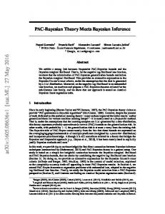
The posterior PDF for the source parameters for a constant priori PDF is proportional to the likelihood function of Equation (4), and it is in this form that we will apply it in the next section. 4 EXAMPLES USING DISPERSION DATA We apply the Bayesian methodology to two dispersion data sets. Firstly, consider source reconstruction for a release in an urban environment. Mean concentration data were extracted from a 30-minute continuous release of sulfur hexafluoride (SF6) tracer in downtown Oklahoma City, Oklahoma, US (Joint Urban 2003 field experiment). We used nine mean concentration data from this release experiment for source reconstruction. The posterior probability of m was calculated, and the resulting posterior PDFs for the source location (xs ,zs ) and emission rate Q are shown in Figure 1. The actual source location was (xs ,zs ) = (3.2506, 1.5537) [expressed in the normalized local coordinate system used by the model] and the true emission rate was Q = 2.00 g s−1 . Both the source location and emission rate are well determined using the Bayesian methodology. The xs and zs locations of the source were estimated to be 3.254 ± 0.019 and 1.559 ± 0.042, respectively; and, the emission rate was estimated to be 1.990 ± 0.041 g s−1 (with the accuracy estimates at one standard deviation). The second example involves source reconstruction for the case of long-range transport using concentration data extracted from the European Tracer Experiment (ETEX) [5]. For the purpose of source reconstruction, we used 35 concentration samples from 10 sampling sites. The posterior PDFs for the source location (in latitudinal and longitudinal coordinates) and the source strength are exhibited in Figure 2. The location of the source was estimated to be at latitudinal and longitudinal coordinates of 47.7◦ ± 0.8◦ N and −2.04◦ ± 1.01◦ E, respectively; and, the emission rate was estimated to be 22.6 ± 2.7 kg h−1 (with accuracy estimates at one standard deviation). The true values for the source location were 48.058◦ N and −2.0083◦ E, and the true emission rate was 28.7 kg h−1 . 5 CONCLUSIONS Bayesian probability theory has been successfully applied to the problem of source reconstruction in the case of pollutant transport and dispersion in complex environments (complex and/or urban terrain involving highly disturbed wind fields exhibiting a significant degree of spatial inhomogeneity and/or temporal non-stationarity). The posterior PDFs of the source parameters for a localized (idealized as a point) source were inferred using measured concentration data from an urban field experiment and the European Tracer Experiment with excellent results. The Bayesian methodology allows optimal estimates of the source parameters to be made along with their reliabilities. 6 ACKNOWLEDGEMENTS The authors wish to acknowledge support from the Chemical Biological Radiological Nuclear Research and Technology Initiative (CRTI) Program under project number CRTI-02-0093RD. 7 REFERENCES 1 H. Ishida, T. Nakamoto and T. Moriizumi, Remote sensing of gas/odor source location and concentration distribution using mobile system, Sensors Actuators B, 49 (1998) 52–57. 2 A. Hehorai, B. Porat and E. Pladi, Detection and localization of vapor-emitting sources, IEEE Trans. Signal Process., 43 (1995) 243–253. 3 T. Flesch, J. D. Wilson and E. Yee, Backward-time Lagrangian Stochastic dispersion models and their application to estimate gaseous emissions, J. Appl. Meteorol., 34 (1995) 1320–1332. 4 L. Robertson and J. Langner, Source function estimate by means of variational data assimilation applied to the ETEX-I tracer experiment, Atmospheric Environment, 32 (1998) 4219–4225. 5 K. Nodop, R. Connolly and F. Girardi, The field campaigns of the European Tracer Experiment (ETEX): Overview and results, 32 (1998) 4095–4108.
Actual source location
1 0.9 0.8
P( Q | D,I)/ P
0
0.7 0.6 0.5 0.4 0.3 0.2 0.1 0 0
1
2
3
4
5
-1 Q (g s )
Figure 1. Posterior probability density function of the source location [left panel] and emission rate (in g s-1) [right panel] for source reconstruction of a continuous point source release in the Joint Urban 2003 experiment.
Actual source location
Figure 2. Posterior probability density function of the source location [left panel] and emission rate (in kg h-1) [right panel] for source reconstruction of a transient point source release in the European Tracer Experiment.