surveillance satellite, in order to prove all possible ... is an Earth low-orbiting geocentric satellite called ... observations memorized on-board in the initial state.
Validation of Decision Models for an Autonomous Earth Surveillance Satellite Florent Teichteil-Königsbuch and Christel Seguin and Cédric Pralet ONERA-DCSD 2 Avenue Édouard-Belin – BP 74025 31055 Toulouse Cedex 4 – France {florent.teichteil,christel.seguin,cedric.pralet}@onera.fr Abstract This paper presents a novel application of Validation and Verification to autonomous decisionmaking. We discuss the relevance of validating formal decision models for an autonomous Earth surveillance satellite, in order to prove all possible on-line decisions are constrained to a given set of validation properties. We distinguish safety and liveness properties depending on whether properties refer to the satellite's physical action dynamics or to the long-term consequences of decisions. We give some examples of both types of properties.
1. Introduction This work deals with the validation of decision models that can be used to control an autonomous spacecraft. Models used for decision planning can have various forms. The paper focuses on a constraints-based model that was designed to optimize the management of the observations made by a geocentric satellite called Frankie. We are investigating ways to validate such models for two main reasons. First, we want to detect subtle potential coding errors as quickly as possible (i.e. use a name of a variable for another). Then, we want also to detect potential misunderstanding or omission of some points of the satellite's mission. To reach these two goals, usual approaches consist in crossing the views on the models. We intend to go a step further than manual independent model inspection. We take advantage of the mathematically well founded form of the model and propose to express expected model properties by another (hopefully) redundant set of constraints. Then we can automatically explore the model and check whether the model is compliant with each property. The paper gives details about this approach, explains how it was practically applied and presents a preliminary set of application results. It is structured
as follows. Section 2 describes the practical application whereas section 3 depicts the studied decision model. Section 4 discusses the kind of properties that can be stated. Section 5 presents how the properties are effectively encoded and assessed. Finally section 6 discusses related and future works.
2. Practical application The AGATA project [1] is a joint CNES (French Space Agency), ONERA (French Aerospace Lab), and LAAS-CNRS (French Robotics Research Center) project, whose objective is to develop tools for improving spacecraft on-board autonomy. This longterm objective covers various fields: the design of control architectures for an autonomous satellite, the design of fault detection identification and recovery capabilities, the development of interaction schemes between the satellite and human ground stations, the development of tools for autonomous decisionmaking, and the use of techniques to validate the satellite behavior. This paper covers the last two aspects, in the sense that it deals with the validation of decision models for an autonomous spacecraft. The satellite considered in the context of AGATA is an Earth low-orbiting geocentric satellite called Frankie. During its successive revolutions, Frankie must make observations defined in a catalog of observations. Observations in the catalog are hot points (volcanic eruptions, forest fires..) detected by an on-board detection instrument, previously identified hot points which must be watched, or observations requested by ground stations. Each observation in the catalog has a given priority degree and can be performed during windows having precise start times, end times, and orientations (the satellite is geocentric but can use a mobile sight mirror to point laterally). Similarly, data can be downloaded to ground stations during predefined visibility slots (download slots). The mission of Frankie is to make observations from the catalog and to download them to ground stations.
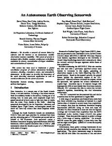
Decision-making capabilities are required since various limitations prevent Frankie from making all observations and from downloading them to the ground. For example, download slots have limited durations, observations which overlap each other are incompatible, energy and memory are limited onboard resources... On-board decisions are made by a mission planning module composed of two interacting components, a reactive one and a deliberative one [2], as shown on Figure 1. The reactive component is in charge of making decisions before action deadlines are met. To choose among the possible decisions, this reactive component can either use a predefined hard-coded strategy, or call the deliberative component. This deliberative component performs reasoning tasks based on a model of the environment and can yield better on-line decisions.
Figure 1: Schema of the interactions between the environment, a reactive task and a deliberative one
3. Decision model The validation process described in this paper concerns the decision model used by the deliberative component of the mission planning module (the reactive component was not validated). This section gives an overview of this decision model, which differs from the more recent model described in a cosubmitted paper [3]. This does not diminish the interest of this work, which is primarily to study validation techniques for decision models.
eclipse or not, observations can already be memorized... In the following, we denote as OBP the set of observations to be performed, as OBM the set of observations memorized on-board in the initial state posted by the reactive component, and as OB the union of these two disjoint sets. Based on these inputs given by the reactive engine each time the deliberative component is invoked, the deliberative component must compute decisions.
3.2. Variables of the decision model The decision model is based on variables over which some constraints hold. All domains of values, including those representing times, are discrete. As described below, variables of the model are of different types. 3.2.1. Temporal variables. In order to handle temporal aspects properly, the decision model focuses on a set of interesting steps, each step i having a certain temporal position t[i] in {0,...,END}. These interesting steps are the steps at which significant changes occur for the satellite, that is the steps at which observations, downloads, or eclipses start or end. It is important to dissociate a step i from its temporal position t[i]. We use auxiliary temporal variables denoted to[i], td[i], and te[i] which represent, at each step i, the next interesting temporal position for the observation, download, and eclipse processes respectively. Planning is performed by choosing a fixed number of steps denoted H in the plans sought. 3.2.2. Decision variables. On-board decisions are represented by a set of decision variables:
3.1. Input parameters The decision model used for validation takes as an input various parameters: a finite temporal horizon [0,..,END] over which the deliberative component must reason to compute decisions; a precise description of observation windows, download slots, and eclipse slots; parameters of the satellite, i.e. the amount of mass memory, the minimum/maximum levels of energy, the angular speed of the mobile sight mirror, power consumptions of the different instruments...; parameters defining the initial state: at the beginning, Frankie can be making observations or downloads, it can be in
obs[i] ∈ {0,1} is a binary decision variable indicating whether the satellite is making an observation at step i. More precisely, obs[i] indicates whether the satellite is making an observation during time interval [t[i],t[i+1][; obsnb[i] ∈ {0} ∪ OBP gives the number of the observations being made at step i (equals 0 if no observation is made at i); dl[i] ∈ {0,1} specifies whether the satellite is downloading some information at step i; ∀ o ∈ OB, dlobs[i,o] ∈ {0,1} takes value 1 if observation o is included in the set of observations being downloaded at step i, 0 otherwise; ∀ o ∈ OBM, fg[o] ∈ {0,1} equals 1 if the satellite decides to forget observation o, 0 otherwise. The satellite can decide to forget an observation initially memorized in order to
release memory and perform higher priority observations. 3.2.3. State variables. Similarly, the state of the satellite is described by several variables: en[i] ∈ {ENmin,..,ENmax} represents the level of energy of the satellite at step i; mem[i] ∈ {0,...,MMmax} is the amount of memory available at step i; ∀ o ∈ OB, memobs[i,o] ∈ {0,1} equals 1 if observation o is memorized on-board at step i; ... Table 1 gives an example of the evolution of the variables previously introduced.
Table 1: variables timeline representation i 0 1 2 3 4 5 t 0 60 80 90 110 150 obs 0 1 1 0 0 0 obsnb 0 8 8 0 0 0 dl 1 1 0 0 0 0 dlobs {1} {1} ecl 0 0 0 0 0 1 memobs {1,2,4} {1,2,4} {2,4} {2,4,8} {2,4,8} {2,4,8} en 65 65 65 65 65 65 mem 232 180 206 206 206 206
6 220 0 0 1 {4,8} 1 {2,4,8} 60 206
7 280 0 0 0 1 {2} 52 250
In this timeline representation [4], we see that at step 0, the satellite is initially downloading observation 1. At step 1, at t[1]=60, the satellite triggers observation 8. This decreases the amount of memory available. Step 2 is the end of the download of observation 1. This observation is therefore not memorized anymore at step 2 and the amount of available memory increases. Step 3 at t[3]=90 corresponds to the end of observation 8. Step 4 at t[4]=110 can be a start time of an observation window, at which the satellite decides not to trigger this observation. Step 5 corresponds to an eclipse start time (ecl[5]=1). At step 6, which is the beginning of a download slot, the satellite chooses to download observations 4 and 8. This download ends at step 7. The energy decreases from steps 5 to 7 since no energy production compensates the platform and instruments consumptions when the satellite is in eclipse.
3.3. Constraints Different kinds of constraints are imposed on the variables of the timelines. A few examples are provided below. Note that the decision model used is completely deterministic and is adapted to a planning/ replanning approach.
3.3.1. Constraints on the temporal variables. t[i+1] = min (to[i],td[i],te[i],END) This constraint states that the time associated with step i+1 is the next important time for one of the three processes (observation, download, eclipse). We do not give the equation of evolution of to[i], td[i], and te[i]. 3.3.2. Constraints on the state variables ((obs[i]=1)∧(obs[i+1]=0)) ⇒ (memobs[i+1,obsnb[i]]=1) ∀ o ∈ OB, ((dlobs[i,o]=1)∧(dlobs[i+1,o]=0)) ⇒ (memobs[i+1,o]=0) ∀ o ∈ OB, (((o≠obsnb[i]) ∨ (obs[i]=0) ∨ (obs[i+1]=1)) ∧((dlobs[i,o]=0) ∨ (dlobs[i+1,o]=1))) ⇒ (memobs[i+1,o] = memobs[i,o])
These constraints express that if an observation finishes at step i+1, then this observation is memorized at i+1, if a download containing observation o finishes at i+1, then o is not memorized anymore at i+1, and in all other situations, the memory content does not vary. en[i+1] = min (ENmax, en[i] + ΔT∙ΔP) where ΔT = t[i+1] - t[i] is the duration between steps i and i+1, and ΔP = (1-ecl[i]) ∙ Psun – obs[i] ∙ Pobs − dl[i] ∙ Pdl − Psat is the power consumption between steps i and i+1. Psun is the power produced by the solar panels, Pobs and Pdl are the power consumed by the observation and download instruments respectively, and Psat is the power consumed by the platform. mem[i+1] = mem[i] dl[i] ∙ (dl[i+1]=0) ∙ ∑(o∈OB) dlobs[i,o].SZ[o] − (obs[i]=0) ∙ obs[i+1] ∙ SZ[obsnb[i+1]] The memory available at i+1 results first from a memory production if a download ends at i+1 (for downloads, the memory is released at the end of the download), and second from a memory consumption if an observation is triggered at i+1 (the memory required to record an observation is consumed at the beginning of the observation). Other constraints describe the evolution of other state variables. 3.3.3. Constraints on the decisions. (obs[i]=1) ⇔ (obsnb[i]≠0) An observation is made at step i if and only if the number of the observation selected at i is not null. ((t[i+1]=to[i]) ∧ (obs[i]=1) ⇒ (obs[i+1]=0)
If step i+1 is interesting for the observation and if the satellite is making an observation at i, this means that this observation ends at i+1, hence obs[i+1]=0.
oversights or clerical errors, like missing parentheses, resulting in a change of constraints' meaning ;
∀ o ∈ OB, (memobs[i+1,o]=0) ⇒ (dlobs[i+1,o]=0)
logical fallacies while translating informal requirements into formal constraints, or while reducing a set of constraints ;
temporal fallacies, due to the violation of long-term consequences or causes of a given property at the present time (it can be a subcase of the previous item).
The satellite can download an observation only if this observation is memorized. Other constraints are enforced, for example, to ensure that the time between two realized observations is sufficient for the sight mirror to move, that the duration of a download does not exceed the duration of the associated download slot, or that observations downloaded are not out of date. 3.3.4. Constraints on the initial and final states. t[0]=0 ecl[0] = ECL0 en[0] = EN0 obsnb[0] = OBSNB0 Other constraints are defined to give an initial value to other state and decision variables. The initial state is assumed to be completely known. The model also imposes constraints on the final state to ensure that at the end of the plan computed, the satellite can reach the next end of an eclipse window with a sufficient level of energy. 3.3.5. Optimization criterion. The optimization criterion chosen is related to the priorities of the observations performed and downloaded. A possible optimization criterion can be to maximize the sum of the values of the observations downloaded and of the observations performed. Other choices are possible.
4. Model's looked-for properties 4.1. Motivation It is not obvious why a formal decision model needs to be validated, since such a model is defined by mathematical constraints that make the model intrinsically satisfy some properties. Actually, most decision model's designers conceive their models as a set of properties that limits the decisions to a set of constrained possible solutions. As a result, if the decision model is not erroneous, all possible decisions are constrained to a safe decision envelope. Nevertheless, we argue we still need to validate the model even if it is formally defined with mathematical constraints: if these constraints are erroneous, there is no chance to prove that the possible solutions are limited to a safe set of decisions. Many mistakes can be made when writing a decision model:
The third item is common to most model-checkers: given a description of the system's dynamics at the present time, is a given property satisfied at all time points (or at one time point) in the future (or in the past)? In other terms, the validation of temporal fallacies checks the consistency of the model over time. Yet, ones may wonder whether it is effective to validate a constraint model, since the validation properties are basically expressed as constraints: if there are mistakes in writing validation constraints – as in writing model's constraints – one may think there is no proof the model is correctly validated, so that validation properties would need to be themselves validated by another validation process, and so on... In fact, the validation of formal decision models can be seen as reformulating the model in a different point of view. In this sense, the validation process can be considered as consolidating each point of view by confronting them each other. As a result, even if validation properties may be erroneous, they are still effective to check potential errors in the model, because they do not strengthen the model's point of view but the reformulated one. If a validation property is not satisfied, it is usually easy to know whether the model or the validation property is wrong. Moreover, in projects involving many people, we think the validation process may be particularly advantageous if persons in charge of decision-making models are not those in charge of validating those models. Indeed, by reformulating the decision model, the latter are able to check that the former have well defined decision-making models. Within project teams, validation is a way to ensure all people are in agreement with the project's requirements. Finally, one may think it suffices to include validation properties in the model, in order to be sure all planner's decisions will satisfy these properties. Nevertheless, we think such approach should not be recommended because redundant validation properties may drastically reduce the planner's running time. Besides, this approach prevents the project's team to analyze any potential model error before the planner is installed on-board the satellite. Errors would be
investigated only after they would occur on-line during the mission.
the next section, we list some liveness properties ; we plan to study the way to validate them in a near future.
4.2. Two kinds of properties We studied two classes of properties: safety properties, and liveness properties [5]. For the studied case, the former must be validated, whereas the latter should be satisfied. 4.2.1. Safety validation properties. Generally speaking, safety properties are model invariants i.e. conditions over system variables that are true at each time step, independently from system past or future. So model invariants are the model constraints that only depend upon the satellite's physical action behavior. They represent the system's internal action dynamics, independently from any decisional artifact like rewards or variables only defined for decision reasoning purposes. Since they enable to check the satellite's physical behavior is not violated, they must be validated. An example set of such properties is validated and discussed in the next section. 4.2.2. Liveness validation properties. Liveness properties mostly require to reach a time step that meets some conditions. In the studied case, these properties refer to the long-term properties of the decision model. They are often used to check that the decision model does not produce dead long-term decisions, like accumulating observations in memory but without downloading them to Earth anytime in the future. As liveness properties are related to decisions but not to model's invariants, their violation can not produce incoherent situations that might endanger the satellite's mission or even itself. Yet, if such properties are not validated, the satellite's decision-maker could produce totally ineffective decisions. Also, liveness properties are in relation to effectiveness but not to safety. In this sense, they should be validated, but it is not an absolute requirement. As liveness properties refer to decisions' long-term effects, it usually makes sense to validate them for infinite-horizon decision models. In our case, the decision model is defined on successive finite horizons, based for instance on eclipse periods, as shown on Figure 2. If a liveness property is not satisfied within one decisional horizon, one expects it will be satisfied within one of the following decisional horizons. In other terms, the violation of a liveness property for a finite model defined for a given time range does not prove at all that this property won't be ever validated in the future (for one of the next finite models). As a consequence, in our finite-horizon case, the validation of liveness properties would require to explore an infinite number of successive finite-horizon decision problems, what we have not yet studied. In
Figure 2: successive finitehorizon planning problems based for instance on alternated eclipse/sunlight periods (same models, but different initial data)
4.3. Model's sensitivity to validation properties By definition, a given property is not validated if and only if there exists a decision that does not satisfy this property. Such a decision is named a counterexample. Since a planner's solution comes from the time-constraint optimization of a numeric criterion, a counterexample does not have to be necessarily optimal. As a consequence, we distinguish two cases for each validation property: there exists a decision that does not satisfy this property (ie a counterexample), what means the planner may on-line produce a counterexample decision;
there does not exist any decision that does not satisfy this property, so that any planner's online possible solution satisfies this property.
In other terms, the validation process aims at proving the second case, i.e. it does not exist any counterexample to each validation property. Besides, it is not certain the on-board planner will produce optimal decisions because of time constraints imposed to deliberative processes. Also, we must prove there does not exist any counterexample independently from the optimization criterion, in order to check all possible planner's (optimal and nonoptimal) solutions. Nevertheless, the optimization criterion associated to each counterexample of a given validation property is a way to assess the model's sensitivity to this property.
5. Implementation with OPL 5.1. Optimization Programming Language OPL (Optimization Programming Language) [6] is a constraint programming language. An OPL problem is defined as a set of logical and numerical constraints, plus a potential optimization criterion. A solution to an OPL problem is an assignment of variables that
satisfy all constraints, and that optimizes a criterion if defined. The AGATA planner we wants to validate is formalized in OPL. The laboratory tests are run with ILOG's OPL Studio.
5.2. Validation property definition in Constraint Programming Let us note the decision model M and any validation property P. The model M is a set of constraints plus an optimization criterion, detailed in section 3. The property P is validated if and only if all (optimal and non-optimal) solutions to M satisfy P. In an equivalent meaning, P is validated if and only if the increased model M∩¬P, but without optimizing the criterion, has no solution. Also, considering the decision model M defined in OPL and a validation property P, we just add the negation of P to M. We then check that this new increased model has no solution, and we eventually report the criterion associated to any potential counterexample. Most validation properties involve first-order logic operators such as and . Since OPL can reinterpret logical values true and false as numerical values 1 and 0 respectively, these operators can be expressed with the OPL operators max and min. Given an arbitrary set S and a boolean function f, it means: s S, f(s) min (s S) f(s)=1 s S, f(s) max (s S) f(s)=1
5.3. Some instances of validated properties In this subsection, we present some safety properties we checked, and some liveness properties we plan to validate in a near future. All properties presented here are validated with the current model. For the first property, we detail its mathematical expression, its negation and its OPL translation. For the others, we only give their mathematical expressions. 5.3.1. Safety properties.
“If an observation is initially forgotten, then it does not exist a step when the observation is downloaded.”
This property is really related to safety, since it is physically impossible to download an observation that is not memorized (because it is initially forgotten). The mathematical constraint expression of this property is: o OBM, fg[o]=1 ⇒ i H, dlobs[i,o]=0 The negation of this property is:
o OBM : fg[o]=1 and i H : dlobs[i,o]=1 The OPL code expressing the latter equation is: max (o in OBM) ((fg(o)=1) & (max (i in H) (dlobs(i,o)=1)))=1;
“At each step, if an observation is being uploaded at this step and if it is not being uploaded at the next step, then it will not being uploaded at any future step.”
This property means that the uploading of observations can not physically be splitted in subtasks, ie between non-adjacent time steps: as soon as an uploading task terminates, it can not be resumed later. The mathematical equation of this sentence is: i H, o OB, (dlobs[i,o]=1 and dlobs[i+1,o]=0) ⇒ j>i, dlobs[j,o]=0
“At each step, if an observation is getting under way and if no uploading is completing, then the memory decreases.”
This property is a way to express the physical behavior of the on-board memory. The situation expressed in this property is one of a few situations where the memory decreases for certain. The related mathematical equation is: i H, i>0 , obs[i-1]=0 and obs[i]=1 and (dl[i-1]=0 or dl[i]=1) ⇒ mem[i] < mem[i-1] 5.3.2. Liveness properties. As mentioned before, our work is not yet mature enough to validate liveness properties, because it would require to take into account successive finite-horizon deliberative processes and the interaction between reactive and deliberative components. For instance, the following properties may not be validated if considered within a single deliberative process, since the reactive process may anytime take control of the immediate decisions upon the deliberative process. As a consequence, validation of liveness properties relies on a subtle and in-depth study of the sequential interleaving of reactive and deliberative processes. Such properties would be:
“At each step, if the set of memorized observations is not empty, then there exists at least one future step when an observation is under way.”
This property is not related to the safety of the model but its liveness, because it formulates that at least one observation will occur. It may be possible that the model is physically correct, but that it prevents the planner to perform any observation.
“At each step, if the energy is minimum, then it exists a future step when the energy is not anymore minimum.”
Again, this is a liveness property, since a physically correct model may lead to decisions which do not recharge the battery when it becomes empty.
“At each step, if at least one observation is memorized, then there exists a future step when an observation is being uploaded.”
This liveness property checks that the decision model gives a chance to observations to be used on ground, in the sense that each observation will be potentially uploaded.
6. Conclusion This paper presented investigations about ways to validate a decision model written in constraint language. The explored issues are manifold. We first tried to identify what could be objective unambiguous assessment criteria and we proposed to express them thanks to additional constraints. Then, we proposed an effective way to check rigorously the expressed properties. We proceeded by refutation i.e. by looking for counterexamples that can invalidate the properties. Finally, we tested the feasibility and the interest of the approach on a concrete example. The approach appeared effective and tractable but the experiment raised a lot of questions. Indeed, a given decision model is a part of a component that contribute to a decision process. So the properties applicable to the model derive both from the requirements applicable to the overall decision process but also from the global decision architecture. This point was more specifically highlighted when dealing with potential liveness properties. It is also worth noting that the properties depend also on the style of the decision models since properties should enable to cross different viewpoints on a same reality. In the presented case, the decision model was centered on the evolution of some parameters rather than on actions. So some proposed properties tend to reconstruct the action view. We have performed a similar exercise on an action based decision model [7] and we observed exactly the dual situation: properties were constrained on timelines. Finally, our experiment shows that it is possible to identify and assess some model properties. The bigger issue now is to study how to derive the most relevant properties from the analysis of the system function and architecture.
7. Acknowledgments The authors would like to thank all people from CNES (French Space Agency), ONERA (French Aerospace Lab), and LAAS-CNRS (French Robotics Research Center) involved in the AGATA project, without whom this research would not have been possible.
8. References [1] Charmeau, M.-C., and Bensana, E. 2005. AGATA: A Lab Bench Project for Spacecraft Autonomy. In Proc. of the 8th International Symposium on Artificial Intelligence, Robotics, and Automation in Space (i-SAIRAS-05). [2] Lemaître , M., and Verfaillie, G. 2007. Interaction between Reactive and Deliberative Tasks for On-line Decision-making. In Proc. of the ICAPS-07 Workshop on “Planning and Plan Execution for Real-world Systems”. [3] Verfaillie, G., Pralet, C., and Lemaître, M. 2007. Constraint-based Modelling of Discrete Event Dynamic Systems. In Proc. of the CP/ICAPS-07 Workshop on “Constraint Satisfaction Techniques for Planning and Scheduling Problems”. [4] Pralet, C., and Verfaillie, G. 2008. Decision upon Observations and Data Downloads by an Autonomous Earth Surveillance Satellite. In Proc. of the 9th International Symposium on Artificial Intelligence, Robotics, and Automation in Space (i-SAIRAS-08). [5] Manna Z. and Pnueli A. 1991. The Temporal Logic of Reactive and Concurrent Systems: Specification. Springer [6] Van Hentenryck, P. 1999. The OPL optimization programming language. MIT Press, Cambridge, MA, USA. [7] Ghallab, M., and Howe, A., and Knoblock, C. and McDermott, D. and Ram, A. and Veloso, M., and Weld, D., and Wilkins, D. 1998. PDDL – The Planning Domain Definition Language. AIPS'08 Planning Committee.