Algorithms and Technologies for Multispectral, Hyperspectral, and Ultraspectral Imagery VIII, N° 4725-54 SPIE AeroSense 2002, 1-5 April 2002, Orlando, FL.
Validation and robustness of an atmospheric correction algorithm for hyperspectral images Yannick Boucher∗, Laurent Poutier, Véronique Achard, Xavier Lenot, Christophe Miesch Office National d’Etudes et de Recherches Aérospatiales, Département d’Optique Théorique et Appliquée ABSTRACT The Optics Department of ONERA has developed and implemented an inverse algorithm, COCHISE, to correct hyperspectral images of the atmosphere effects in the visible-NIR-SWIR domain (0,4-2,5 µm). This algorithm automatically determine the integrated water-vapor content for each pixel, from the radiance at sensor level by using a LIRR-type (Linear Regression Ratio) technique. It then retrieves the spectral reflectance at ground level using atmospheric parameters computed with Modtran4, including the water-vapor spatial dependence as obtained in the first step. The adjacency effects are taken into account using spectral kernels obtained by two Monte-Carlo codes. Results obtained with COCHISE code on real hyperspectral data are first compared to ground based reflectance measurements. AVIRIS images of Railroad Valley Playa, CA, and HyMap images of Hartheim, France, are used. The inverted reflectance agrees perfectly with the measurement at ground level for the AVIRIS data set, which validates COCHISE algorithm. For the HyMap data set, the results are still good but cannot be considered as validating the code. The robustness of COCHISE code is evaluated. For this, spectral radiance images are modeled at the sensor level, with the direct algorithm COMANCHE, which is the reciprocal code of COCHISE. The COCHISE algorithm is then used to compute the reflectance at ground level from the simulated at-sensor radiance. A sensitivity analysis has been performed, as a function of errors on several atmospheric parameters and instruments defaults, by comparing the retrieved reflectance with the original one. COCHISE code shows a quite good robustness to errors on input parameters, except for aerosol type.
1. INTRODUCTION Most applications of hyperspectral imagery need atmospherically corrected data. The Optics Department of ONERA has developed an algorithm for the atmospheric correction of hyperspectral images in the visible-NIR-SWIR domain (0,4-2,5 µm). This algorithm is called COCHISE (COde de Correction atmosphérique Hyperspectrale d’Images de Senseurs Embarqués: atmospheric correction code for hyperspectral images of remote-sensing sensors). It permits to compute the spectral reflectance at ground level and determine automatically the integrated water-vapor content of each pixel, from a calibrated hyperspectral radiance image at sensor level. COCHISE code is first described in detail in section 2. Section 3 presents some results obtained with COCHISE code on real hyperspectral images. Two data set have been proceeded: AVIRIS images on Railroad Valley Playa, CA, and HyMap images of Hartheim, France (DAISEX’99 campaign). The inverted reflectances are compared to reflectance ground measurements for both data sets. Section 4 is devoted to the evaluation of the robustness of COCHISE code. The method uses simulated spectral radiance images at sensor level, computed with the direct algorithm COMANCHE (COde de Modélisation pour l ’ANalyse des Cibles Hyperspectrales vues en Entrée instrument: Code for the analysis of hyperspectral targets signatures at sensor ∗
[email protected]; phone: (33) 562 25 26 26; fax: (33) 562 25 25 88; URL: http://www.onera.fr/dota-en/; ONERA Centre de Toulouse, DOTA, BP 4025, 31055 TOULOUSE CEDEX 4, FRANCE
2
entrance level). COCHISE code is then used to compute the ground reflectance from the simulated radiance with COMANCHE. Errors on several input parameters like aerosols type and content, instrument noise, instrument calibration errors and presence of liquid water absorption bands in the reflectance spectra, are firstly introduced. The inverted reflectance is then compared to the original one, with criteria like root mean square error and spectral angle.
2. DESCRIPTION OF COCHISE ALGORITHM The aim of COCHISE atmospheric correction code is to compute the intrinsic optical properties of a landscape from the data delivered by an airborne or spaceborne calibrated hyperspectral sensor. The available wavelength domain of COCHISE is the VIS-NIR-SWIR domain (0.4-2.5 µm), since the emissive compound of the signal is not taken into account. Thus, the reflectance at ground level is calculated for each spectral band in this domain. COCHISE also permits to compute automatically the integrated water-vapor content for each pixel, to limit the requirement to exogenous data. The chosen analytical formulation of upwelling radiance at sensor entrance pupil level L tot (x, y, λ ) , similar to the formulation of 6S1, separates atmospheric parameters from the ground parameters:
L tot (x, y, λ ) = L atm (λ ) + t dir (λ ) ⋅ Lp0 (x , y, λ ) + t dif (λ ) ⋅ Lenv 0 (x , y, λ )
(1)
L atm (λ ) models the atmospheric radiance, with no interaction with the ground surface. The second term models the upwelling radiance directly transmitted from the ground. It is the product of the direct transmission t dir (λ ) from the ground surface to the sensor, by the upwelling radiance Lp0 (x, y, λ ) of the pixel at the ground level. The third term models the environment effects. It is the product of the diffuse upwelling transmittance t dif (λ ) and the upwelling
radiance of the pixel environment at the ground level, Lenv 0 (x , y, λ ) . This decomposition is represented in Fig. 1. sensor
IFOV
Latm (λ) t dir (λ)Lp0 (λ)
t dif (λ)Lenv 0 (λ)
ρG ρF background
pixel
Fig. 1: Illustration of the contributors of the pixel upwelling radiance.
For the following, the ground surface is assumed flat and lambertian. This is a strong hypothesis, but necessary in the perspective of the inversion of equation (1). This assumption is usually made in most of atmospheric correction algorithms2,3,4. The upwelling radiance of the pixel at ground level can be written5:
3
Lp0 (x , y, λ ) =
E 0 ⋅ ρ(x, y, λ ) π ⋅ [1 − ρ G (x, y, λ ) ⋅ S(λ )]
(2)
Where E0(λ) is the downwelling irradiance (without taking into account the trapping effects due to ground reflexion), ρ(x,y,λ) is the spectral albedo of the considered pixel, ρ G (x, y, λ ) an average albedo taking into account the adjacency effects due to ground reflexion, and S(λ) the spherical albedo of the atmosphere. The upwelling radiance at ground level due to the environment can be written following a similar formulation7:
Lenv 0 (x , y, λ ) =
E 0 ⋅ ρ F (x, y, λ ) π ⋅ [1 − ρ G (x , y, λ ) ⋅ S(λ )]
(3)
Where ρ F (x, y, λ ) is the averaged albedo due the scattering towards the sensor of light reflected by the environment. The albedos ρF and ρG are obtained by the convolution in the spatial domain of the pixel albedo with spectral kernels depending on background reflectance and atmosphere properties. For each λ:
ρ F (x , y, λ ) = ρ(x , y, λ ) ⊗ Fλ (x, y )
(4)
ρG (x, y, λ ) = ρ(x , y, λ ) ⊗ G λ (x , y )
(5)
Fλ(r) represents the probability that a light ray reflected by the environment of the pixel at a distance r from the center of the pixel, would be scatterd by the atmosphere towards the sensor IFOV. Gλ(r) represents the probability that a light ray that finally reaches the pixel of interest after trapping effects, would have it last interaction with the ground at a distance r from the center of the pixel. COCHISE algorithm consists in inverting equation (1) combined with equation (2) and (3), thanks to an iterative method. The wanted pixel albedo may be written:
ρ(x, y, λ ) =
1 − ρ G (x, y, λ ) ⋅ S(λ ) π ρ F (x , y ) ⋅ ⋅ L tot (x, y ) − L atm − t dif ⋅ t dir 1 − ρ G (x, y, λ ) ⋅ S(λ ) E0
(
)
(6)
In a first step, the environmental functions are neglected, and ρF and ρG are supposed to be equal to ρ. The first estimate of the pixel albedo is thus obtained by:
ρˆ (x, y, λ ) =
L tot (x , y, λ ) − L atm (λ ) E 0 (λ ) ⋅ [t dir (λ ) + t dif (λ )] + S(λ ) ⋅ L tot (x, y, λ ) − L atm (λ ) π
[
]
(7)
Environment albedos ρˆ F (x, y, λ ) and ρˆ G (x, y, λ ) are then calculated from equations (4) and (5), and reinjected in equation (6). The environment functions Fλ(r) and Gλ(r) are preprocessed with a Monte Carlo method, adapted from AMARTIS radiative transfer code5, 6. This second iteration gives satisfactory results. Meanwhile, a more accurate convergence could be obtained by other iterations, if necessary. The spectral atmospheric parameters tdir(λ), tdif(λ), E0(λ), Latm(λ) and S(λ) are also pre-computed, using MODTRAN47 with different ground reflectance conditions5 (ρ=0, ρ=0.5 and ρ=1) and for a set of water-vapor contents corresponding to the amounts estimated in a prelimininar stage. The water-vapor retrieval is based on a look-up table (LUT) of a linear regression ratio8 RLIRR(ρ,w), depending on reflectance ρ and water-vapor integrated content w, is also pre-computed:
R LIRR (ρ, w ) =
Lm LIR (λ r , L r )
(8) λm
4
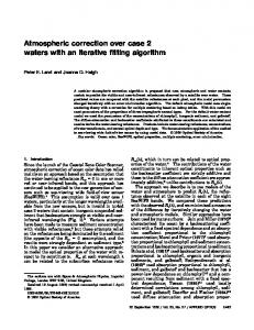
Where Lm are the radiance values in the measurement channel (water-vapor absorption band), and LIR the radiance obtained by linear regression on the radiance values in the reference channels, at the average measurement wavelength λ m (see Fig. 2 ). Radiance Lri LIR = b.λρ + c Lrj Lm λri
λm
λrj
Wavelength
Fig. 2: Illustration of the LIR Ratio determination method for the estimation of water vapor content
The LIRR is computed for each pixel from the radiances in reference and measurement channels, so that the columnar water vapor amount can be determined with the LUT on a pixel by pixel basis.
3. VALIDATION WITH HYPERSPECTRAL IMAGES AND GROUND TRUTH A preliminary validation has been performed by the comparison of COCHISE with some radiative transfer reference codes5, and is out of the scope of this paper. It has been shown that the environment effects were modeled in a satisfying way. The coherence between COCHISE and COMANCHE has also been verified for various atmospheric and reflectance conditions. Some images were simulated with COMANCHE code for various aerosol types, visibility or ground components, and inverted with COCHISE. In most of cases, the agreement between original reflectance and retrieved one is very good (RMS error smaller than 1%). The water vapor content is also retrieved with a very good precision. The maximum errors occur when the ground reflectance spectra contain liquid water absorption bands. In this case, uncertainties on water vapor retrieval increase and the RMS error is approximately 3% on the entire spectra. These results have proved the capacity of COCHISE to retrieve the ground reflectance and water vapor content, and are not presented here. We emphasize in this paper on the validation of COCHISE with hyperspectral experimental data sets including the acquired radiance hypercubes, ground-truth measurements of spectral reflectances and a description of the atmospheric characteristics involved in the radiative transfer. This validation is based on the comparison of reflectance spectra retrieved by COCHISE, from real hyperspectral images, and ground-based reflectance measurements. Thus, high quality hyperspectral images have been chosen, from the airborne hyperspectral sensors AVIRIS9 and HyMap10. 3.1 Inversion of AVIRIS data The data set is composed of an AVIRIS radiance hypercube (0.369-2.51µm, 224 bands) acquired on the Railroad Valley Playa the 17 June 1998, and ground truth data: a reflectance spectrum of the ground measured in the field with an ASD Fieldspec spectrometer, and atmospheric characteristics including optical depths at different wavelengths. These last data sets allow to determine the aerosol behavior. The results are presented for a 100x100 pixels region of the original AVIRIS image. The pixel size at ground level is approx. 20mx20m. Fig. 3 represents the retrieved reflectance image in the band #26 (0.616µm), and in the band #132 (1.604µm). Two blue tarps were set up on the ground, that can be seen on the reflectance image (band #26) as two dark points in the center of the image. This two tarps delimitate the zone where ground measurements were performed. The tarps are not visible in the infrared (band #132) and the image presents less contrast.
5
Fig. 3: Reflectance image (left: band #26 0.662 µm, right: band #132, 1.604 µm) retrieved with COCHISE on a 100x100 pixels region of the Railroad Valley Playa AVIRIS image
The reflectance retrieved spectrum of a 45 pixels zone between the tarps is plotted on Fig. 4. The error bars on retrieved spectrum represent the minimum and maximum values on the 45 pixels zone. The error bars on the ground measurements (appearing in light grey pattern) represent the measurement uncertainty (standard deviation). The agreement is very good in most of spectral bands, since the error bars of the two spectrum intersected themselves. One can see that even in 0.94 and 1.13 µm absorption bands, the results remain quite good. The most important disagreement happens below 0.4µm, that may be explained by the low radiance values in these bands, and by the Noise Equivalent delta Radiance (NedL) of AVIRIS, that dramatically increases under 0.4µm11. The AVIRIS calibration is also less accurate in this domain for the same reasons. 0,7
Reflectance
0,6 0,5 0,4 0,3 0,2 Ground truth 0,1
COCHISE retrieval
0 0,3
0,5
0,7
0,9
1,1
1,3
1,5
1,7
1,9
2,1
2,3
2,5
wavelength (µm) Fig. 4: COCHISE retrieved reflectance spectrum and ground-based reflectance measurement of the Railroad Valley Playa reference zone
The water-vapor image retrieved with COCHISE and the corresponding histogram are presented on Fig. 5. The watervapor image is quite uniform, except for the relief areas on the left corner of the image. The mean value of water vapor content in the area of interest is 0.99 g/cm2, while the measured original value is 1.3 g/cm2. This difference could be partly explained by the fact that COCHISE retrieves water vapor amounts in a L-shape path from the sun, through the ground and up to the sensor, whereas the ground truth is obtained by a vertical radiosounding on a slightly different area. This point is still under investigation.
6
Fig. 5: Water vapor image of Railroad Valley Playa retrieved with COCHISE (left), and corresponding histogram (right)
Except for the water-vapor retrieval content, the results obtained with COCHISE from AVIRIS Railroad Valley Playa image fit with a very good precision the ground truth reflectance measurements. 3.2 Inversion of HyMap data This data set is composed of an HyMap radiance hypercube (0.45-2.48µm, 128 bands) acquired on Hartheim, France, the 17 July 1999, in the DAISex99 experiment.
Fig. 6: Reflectance image (left: band #17, 0.671 µm, right: band #80, 1.606 µm) retrieved with COCHISE on a 121x121 pixels region of the Hartheim HyMap image
The altitude of the flight was 2740m, so that the pixel size at ground level was 6.3x5.1m. The region of interest was a coniferous forest. The reflectance of the canopy was measured with an ASD Fieldspec spectroradiometer, from a truckmounted platform (10m height), thanks to a spectralon reference panel. The used atmospheric profile was supplied by the AVISO meteorological analysis (0.25° mesh) from Meteo-France.
7
The results of COCHISE inversion are presented for a 121x121 pixels region of interest of the original HyMap image. Fig. 6 represents the retrieved reflectance image in band #17 (0.671µm), and in band #80 (1.606µm).
0,3 0,25
Ground measurement
Reflectance
COCHISE retrieval
0,2 0,15 0,1 0,05 0 0,3
0,5
0,7
0,9
1,1 1,3 1,5 1,7 wavelength (µm)
1,9
2,1
2,3
2,5
Fig. 7: COCHISE reflectance retrieved spectrum and ground-based reflectance measurement spectrum of the Hartheim reference zone
Fig. 8: Water vapor image of Hartheim site retrieved with COCHISE (left), and corresponding histogram (right)
The retrieved reflectance spectrum of the top of the canopy is plotted on Fig. 7. The agreement between the computed reflectance and the ground measurement is better than 10% over almost all the spectral domain. However, results are not as good as those obtained with the AVIRIS data set. The first reason is the difference between the two airborne imaging spectrometers. Although its high signal to noise ratio10, we do not have a precise idea of HyMap calibration quality for this flight. The second reason is the lower reflectance of coniferous canopy of Hartheim forest in front of sand reflectance of Railroad Valley Playa. Thus, the radiance is 3 to 5 times weaker for the Hartheim image, depending on the spectral band. Finally, the spectral reflectance measurement at ground level is far more difficult for the forest than for the sand. Indeed, the sand is almost lambertian, while directional effects and structural effects are more
8
pronounced for the forest. The measurement itself is more difficult since the spectralon reference panel was not at the same distance from the spectrometer as the canopy. At last, no uncertainty is supplied with this reflectance data set. All these points may explain the differences obtained. The water-vapor image retrieved with COCHISE and the corresponding histogram are presented on Fig. 8. The histogram statistics have been computed on the center of the image, and do not include the liquid water zone visible in the top-right part of the image. The water-vapor image is rather uniform. The value of water vapor content retrieved with COCHISE in the area of interest is 1.62 g/cm2, while the value obtained from the AVISO profile is 1.81 g/cm2. As for AVIRIS image this underestimation of water vapor content is still under investigation. The results obtained with COCHISE from the HyMap image of Hartheim forest agree with the ground reflectance measurements, taking into account the complexity of the surface canopy and the uncertainty on data quality.
4. ROBUSTNESS OF COCHISE TO INSTRUMENT DEFECTS AND ERRORS ON ATMOSPHERIC PARAMETERS The object of this section is to evaluate the robustness of COCHISE code towards input parameters errors. Indeed, except for the water vapor content automatically computed, other atmospheric parameters are needed as input data. The evaluation of COCHISE performances thanks to known errors on input parameters is representative of the robustness of this code. In the same way, the sensitivity of COCHISE performances to instrumental or calibration errors is interesting, since instruments are never perfect. The study was performed by using successively COMANCHE and COCHISE. COMANCHE was first used to model uniform radiance images corresponding to HyMap spectral bands. The model implemented in COMANCHE is based on equations (1) to (3) and is described elsewhere5. The ground reflectance and water vapor were retrieved from the simulated hyperspectral image by using COCHISE, after having voluntarily introduced some errors on COCHISE input parameters. Radiance images are computed with a middle latitude summer atmospheric profile and the water vapor content is equal to 2.94 g/cm2. The original reflectance and the reflectance inverted with COCHISE are compared using three criteria: r r ρo ⋅ρc Spectral angle: SA = Arc cos r r ρ .ρ o c
Root Mean Square error σrms:
σ rms =
Relative root Mean Square error σr: σ r =
1 Nλ
1 Nλ
Nλ
∑ (ρ 0 (λ i ) − ρ c (λ i ))2 i =1
ρ 0 (λ i ) − ρ c (λ i ) ρ 0 (λ i ) i =1 Nλ
∑
2
Where ρ0 is the original reflectance spectrum, and ρc the reflectance spectrum computed with COCHISE from radiance images simulated with COMANCHE. 4.1 Robustness of COCHISE to instrument defects A vegetation reflectance spectrum has been chosen to create radiance images. This spectrum contains liquid water absorption bands and many spectral variations, which represents actually an unfavorable case. The influence of radiometric noise is firstly investigated. Two kinds of noise have been added on radiance images. The first one is proportional to signal (a random function between +/- 1% of radiance) and the other one is a random function between +/-0.05 W/µm/m2/sr added to signal. These noises are compatible with the HyMap signal-to-noise ratio. Due to radiometric noise, retrieved water vapor content varies on radiance images. Added radiometric noise is
9
weak in relation to measured signal in the 940 nm water vapor spectral band, so its influence on water vapor content retrieval is lower than proportional noise. Inversion remains accurate in presence of this kinds of noise. One can see on Fig. 9 that the error is very weak.
___ ___
ρ original ρ retrieved
___ ___
wavelength
SA = 0.0099
σrms = 0.0035
ρ original ρ retrieved
wavelength
σr = 0.0179
SA = 0.008
σrms = 0.0080
σr = 0.041
Fig. 9: Water vapor content graph and reflectance spectra obtained with COCHISE, with noise added to the radiance signal (+/- 1% of the radiance on left and +/- 0.05 W/µm/m2/sr on right)
The robustness to uncertainties on spectral calibration is now evaluated. HyMap spectral bands are positioned with a 0.5 nm accuracy. The spectral bands defined in COMANCHE are shifted by +/- 0.5nm in COCHISE: • with the same shift for all bands (+0.5 nm or –0.5 nm) • with a random shift included between –0.5 nm and + 0.5 nm A spectral random shift can locally influence inversion, especially when an important shift appears on measurement bands used to retrieve columnar water vapor content. So this process has been repeated several times to cover all patterns. The worst results obtained are presented Fig. 10. The highest error appears with the constant shift. There is a 3% error on the water vapor content which creates a small error on the water vapor correction. There is also a 3% RMS error on the entire spectra which doesn’t affect significantly the inversion results. An inversion with all combined instrument defects is then studied. Both spectral and radiometric defects have been applied to the radiance spectrum to perform the inversion. However, except in the strong water vapor absorption bands, inversion results are quite satisfactory (Fig. 11).
10
___ ___
ρ original ρ retrieved
___ ___
wavelength
SA = 0.0185 H2O = 3.03 g/cm2
ρ original ρ retrieved
wavelength
σrms = 0.0067 σr = 0.033
SA = 0.0184 H2O = 3.03 g/cm2
σrms = 0.0072 σr = 0.028
Fig. 10: vegetation reflectance spectra obtained by COCHISE with spectral shift. On the left, inversion is performed with a constant shift and on the right, with a random shift.
___ ___
ρ original ρ retrieved
wavelength
SAM = 0.0284
σrms = 0.010
σr = 0.032
Fig. 11: water vapor content graph and vegetation reflectance spectra obtained by COCHISE with all instrument defects (two types of noise and spectral random shift)
4.2 Robustness to errors on atmospheric input parameters This analysis has been performed with a 0.5 constant reflectance spectrum in order to see the impact of the ignorance of some atmospheric parameters, and particularly those related to aerosols, on the retrievals at each wavelength. The impact of an error on atmospheric visibility is firstly investigated. Visibility expresses atmospheric opaqueness and influences atmospheric radiance and both direct and diffuse transmittances. Low visibility induces weak direct transmittance and high diffuse transmittance. At the opposite, high visibility induces great direct transmittance and weak diffuse transmittance. The COMANCHE visibility was 23 km then COCHISE was run respectively with a lower (15 km) and a higher (30 km) visibility. The retrieved reflectance are weakly influenced by such an error. In fact, reflectance is under-estimated when visibility is overestimated and vice-versa (Fig. 12). Then the impact of a wrong aerosol type is evaluated. Both composition and particle size vary with aerosol type. Particle size affects diffusion phenomena, which are especially important in visible spectral domain. This simulation has been performed by using rural aerosol type to compute radiance images. Inversion was realized with a maritime or urban aerosol type (Fig. 13). For the maritime aerosol case, the retrieved reflectance spectrum is weakly erroneous. Inversion error is greater in the second case (urban aerosols): reflectance average value is overestimated and reflectance
11
spectrum shape has changed. Reflectance spectrum is curved with a 15% maximal error on spectrum ends. Thus, a good knowledge of aerosol type is necessary to perform an accurate inversion.
___ ___
ρ original ρ retrieved
___ ___
wavelength
SAM = 0.0137 H2O = 2.79 g/cm2
ρ original ρ retrieved
wavelength
σrms = 0.0087 σr = 0.017
SAM = 0.0108 H2O = 2.99 g/cm2
σrms = 0.0057 σr = 0.011
Fig. 12: Reflectance spectra obtained by COCHISE with visibility error. COMANCHE is used with a 23 km visibility and inversion is performed with a 15 km visibility (on the left) or with a 30 km visibility (on the right)
___ ___
ρ original ρ retrieved
___ ___
wavelength
SAM = 0.0147 H2O = 2.78 g/cm2
ρ original ρ retrieved
wavelength
SAM = 0.0239 H2O = 2.99 g/cm2
σrms = 0.0098 σr = 0.020
σrms = 0.033 σr = 0.067
Fig. 13: Inversion performed with a wrong aerosol type but the right visibility (23km): Maritime aerosol type (left) and urban aerosol type (right) are used instead of rural aerosols.
5. SUMMARY COCHISE code allows to perform an atmospheric correction of hyperspectral images in the visible-NIR-SWIR domain (0,4-2,5 µm). The algorithm is based on a simple analytical formulation of the radiance at the sensor level, which separates the atmospheric contributors from the ground reflection properties. The inversion is performed with an iterative method taking into account the adjacency effect in the second iteration, using convolution kernels obtained with two Monte-Carlo codes that simulate the trapping effects and the spread out of the upwelling transmittance. The radiative transfer is computed using Modtran4, and the water-vapor content with a LIRR-type (Linear Regression Ratio) technique. COCHISE code has been used to inverse an AVIRIS hypercube on Railroad Valley Playa. The retrieved reflectance spectrum has been compared to ground-based reflectance measurements. The measured and inverted spectra are in a
12
very good agreement. A Hymap data set on Hartheim forest, France, has also been proceeded, and COCHISE results compared to ground reflectance measurements. The differences between the measured and the inverted spectrums are around 10%, and are explained by the scene variability, the directional and structural effects of the canopy and the measurements uncertainties. For both data sets, the retrieved water vapor contents are underestimated of 10 to 30%; this point is still under investigations. The robustness of COCHISE code as been evaluated with simulated hyperspectral images. A sensitivity analysis has been performed, as a function of errors on COCHISE input parameters. COCHISE code shows a good robustness to the instrument defects like noise and error on spectral calibration. The robustness to errors on atmospheric parameters is good for reasonable error on visibility, but an error of aerosol type introduces a non-negligible bias. Finally, COCHISE atmospheric correction code for hyperspectral images in the VIS-NIR-SWIR domain is validated and presents a good robustness on input parameters errors.
ACKNOWLEDGEMENTS The works presented are supported by the DGA, DSP/STTC/OP (Délegation Générale de l’Armement, Direction des Systèmes de forces et de la Prospective, Service Technique des Technologies Communes, Département Optronique). AVIRIS data on Railroad Valley Playa and ground-based measurements are courtesy of K. Thome, Optical Science Center, Remote Sensing Group, University of Arizona. DAISEX’99 data including HyMap image on Hartheim are courtesy of Patrick Wurteisen, European Spatial Agency; many thanks to Marc-Phillipe Stoll and Françoise Nerry, LSIIT, for the supplying of the data.
REFERENCES 1.
E. Vermote., D. Tanré, J.L. Deuzé, M. Herman, J.J. Mocrette, “Second Simulation of the Satellite Signal in the Solar Spectrum (6S)”, 6S User Guide Version 2, 1997. 2. A. F. Goetz, J.W. Boardman, B. Kindel and K.B. Heidebrecht, Atmospheric corrections: On deriving surface reflectance from hyperspectral imagers, Proceedings SPIE Annual Meeting, 3118, 14-22, 1997. 3. Zheng Qu, Alexander F. H. Goetz, and Kathleen Heidebrecht, “High-Accuracy Atmosphere Correction for Hyperspectral Data (HATCH)” 2000 AVIRIS Earth Science and Applications Workshop Proceedings, 2000. 4. S. Adler-Golden,, A. Berk, L.S. Bernstein, S. Richtsmeier, P.K. Acharya, M.W. Matthew, G.P. Anderson, C.L. Allred, L.S. Jeong, J.H. Chetwynd, “FLAASH, a Modtran4 atmospheric correction package for hyperspectral data retrievals and simulations”, 1998 AVIRIS Earth Science and Applications Workshop Proceedings, 1998. 5. L. Poutier, C. Miesch, X. Lenot, V. Achard, Y. Boucher, “COMANCHE and COCHISE”: two reciprocal atmospheric codes for hyperspectral remote sensing”, 2002 AVIRIS Earth Science and Applications Workshop Proceedings, 2002. 6. C. Miesch, X. Briottet, Y. Kerr, F. Cabot, “Radiative transfer solution for rugged and heterogeneous scene observations”, Applied Optics, Vol. 39, No.36, pp. 6830-6846, 20 December 2000. 7. G. Anderson, A. Berk, P.K. Acharya, M.W. Matthew, L.S. Bernstein, J.H. Chetwynd, H. Dothe, S.M. AdlerGolden, A.J. Ratkowski, G.W. Felde, J.A. Gardner, M.L. Hoke, S.C. Richtsmeier, B. Pukall, J. Mello, L.S. Jeong, 2000, “MODTRAN4 : Radiative transfer modeling for remote sensing”, Algorithms for Multispectral, Hyperspectral, and Ultraspectral Imagery VI, Proceedings of SPIE, Vol. 4049, pp. 176-183. 8. D. Schläpfer D., K. Itten, “Imaging spectrometry of tropospheric ozone and water vapor”, EARSeL Int. J. ‘Advanced in Remote Sensing’, 1995. 9. R. Green, M. Eastwood, C. Sarture, “Imaging spectroscopy and the Airborne Visible Infrared Imaging Spectrometer (AVIRIS)”, Remote Sens. Environ., Vol. 65 n°3, pp. 227-248, Sept. 1998. 10. T. Cocks, R. Jenssen, A. Stewart, I. Wilson, T. Shields, “The HyMap airborne hyperspectral sensor: the system, calibration and performance”, 1st EARSEL Workshop on imaging spectroscopy, Zurich, Oct. 1998. 11. R. Green, B. Pavri, “AVIRIS In-flight calibration experiment, sensitivity analysis, and intraflight stability”, Proc. Of the 9th JPL Airborne Earth Science Workshop, p. 207, Dec. 2000.