Validation of Vector Data using Oblique Images Pragyana Mishra
Eyal Ofek
Gur Kimchi
Microsoft Corporation One Microsoft Way Redmond, WA 98052 +1 425 421 8518
Microsoft Corporation One Microsoft Way Redmond, WA 98052 +1 425 706 8866
Microsoft Corporation One Microsoft Way Redmond, WA 98052 +1 425 722 2050
[email protected]
[email protected]
[email protected]
ABSTRACT Oblique images are aerial photographs taken at oblique angles to the earth’s surface. Projections of vector and other geospatial data in these images depend on camera parameters, positions of the entities, surface terrain, and visibility. This paper presents a robust and scalable algorithm to detect inconsistencies in vector data using oblique images. The algorithm uses image descriptors to encode the local appearance of a geospatial entity in images. These image descriptors combine color, pixel-intensity gradients, texture, and steerable filter responses. A Support Vector Machine classifier is trained to detect image descriptors that are not consistent with underlying vector data, digital elevation maps, building models, and camera parameters. In this paper, we train the classifier on visible road segments and non-road data. Thereafter, the trained classifier detects inconsistencies in vectors, which include both occluded and misaligned road segments. The consistent road segments validate our vector, DEM, and 3-D model data for those areas while inconsistent segments point out errors. We further show that a search for descriptors that are consistent with visible road segments in the neighborhood of a misaligned road yields the desired road alignment that is consistent with pixels in the image.
Categories and Subject Descriptors I.4.8 [Image Processing and Computer Vision]: Scene Analysis – Surface fitting.
General Terms Algorithms
Keywords Computer vision, Machine learning, Mapping, Vector data, Pixel statistics, Oblique image analysis, Multi-cue integration, Conflation.
1. INTRODUCTION Generating a map may involve several sources of information—a few of which include vector data, map projection parameters, digital elevation maps (DEM’s), and 3-dimensional (3-D) models. Permission to make digital or hard copies of all or part of this work for personal or classroom use is granted without fee provided that copies are not made or distributed for profit or commercial advantage and that copies bear this notice and the full citation on the first page. To copy otherwise, or republish, to post on servers or to redistribute to lists, requires prior specific permission and/or a fee. ACM GIS '08 , November 5-7, 2008. Irvine, CA, USA. © 2008 ACM ISBN 978-1-60558-323-5/08/11...$5.00
Errors or inaccuracies in these data sources contribute to the overall accuracy and quality of the map. Detecting these errors is difficult as there is little or none ground truth available against which the data can be compared to. Most aerial and satellite images that may be used as ground truth for data validation are nadir views of the world. However, the set of attributes of data that can be validated using aerial images is limited. This is due to the fact that the projection is orthographic in nature and 3-D—both terrain and building structuredependent—attributes of the scene are not entirely captured in nadir orthographic views. Inaccuracies in altitude, heights of buildings, and vertical positions of structures cannot be easily detected by means of nadir imagery. These inaccuracies can be detected in an image where the camera views the scene at an oblique angle. Oblique-viewing angles enable registration of altitude-dependent features. Additionally, oblique viewing angles bring out the viewdependency of 3-dimensional geospatial data; occluding and occluded parts of the world are viewed in the image depending on the position and orientation at which the image was taken. Image pixel regions that correspond to occluding and occluded objects can be used to derive consistency of the geospatial entities as they appear in the image. The consistency can be further used to rectify any inaccuracies in data used for segmenting and labeling of the objects. Oblique images are aerial photographs of a scene taken at oblique angles to the earth’s surface. These images have a wide field of view and therefore, cover a large expanse of the scene as can be seen in Figures 4 through 7. Oblique images capture the terrain of earth’s surface and structures such as buildings and highways. For example, straight roads that are on the slope of a hill will appear curved. The mapping between a 3-D point of the world and its corresponding point on the image is a non-linear function that depends on the elevation, latitude, and longitude of the 3-D point in space. Additionally, visibility of the 3-D point depends on the camera’s position and orientation, and the structure of the world in the neighborhood of that 3-D point; the point may not be visible in the image if it is occluded by a physical structure in the line-ofsight of the camera. These properties can, therefore, be used to detect and rectify any errors of the 3-D point’s position as well as any inconsistencies of structures in the neighborhood of the point. Pixels of oblique images can be analyzed to detect, validate, and correct disparate sources of data, such as vectors, projection parameters of camera, digital elevation maps (DEM’s), and 3-D models. This is a novel use of oblique imagery wherein errors due
to inaccurate and imprecise vectors, DEM, map projection parameters, and 3-D model data are detected and rectified using pixel statistics of oblique images. We present a statistical-learning algorithm to learn image-based descriptors that encode visible data consistencies, and then apply the learnt descriptors to classify errors and inconsistencies in geospatial data. The algorithm combines different descriptors such as color, texture, imagegradients, and filter responses to robustly detect, validate, and correct inconsistencies.
2. OBLIQUE IMAGES Oblique images capture the view-dependency and height of geospatial data. This unique characteristic makes oblique images ideal for validation and correction of disparate data sources. The projection of the 3-D world accounts for altitude (terrain), structure models, and the arrangement of geospatial entities with respect to each other. Both the horizontal and vertical attributes, which are visible in oblique views, can be used to constrain the set of possible hypotheses for generating attributes of geospatial data. Vertical attributions such as visible building facets can be used to validate geospatial structures and models. The advantages of using oblique views over nadir views are discussed in the research on generating 3-D building models from monocular aerial images [1][2]. The oblique angle, i.e. the angle formed by the optical axis of the camera with respect to the Z-axis of the world coordinate system, of our oblique images varies between 30 to 45 degrees. This falls in the category of high oblique photography. In photogrammetry, a nadir or vertical image has a small tilt angle, typically on the order of five degrees; a low oblique image is considered to be one that has between 5 and 30 degrees of tilt, and high oblique image has greater than 30 degrees of tilt [2]. The term oblique image refers to a high oblique image in this paper. In order to understand and learn appearances of 3-D geospatial entities as observed in images, image-pixel statistics are first computed using a set of descriptors. A SVM classifier is then trained for learning these descriptors. The classifier validates points that are consistent with learnt descriptors for a given geospatial entity and detects those that are not. In this paper, the chosen geospatial entity is road data. However, our classifier can be trained to detect consistency of other geospatial entities such as buildings, water bodies, foliage, parking lots, and railway lines.
3. IMAGE DESCRIPTORS Image descriptors encapsulate pixel statistics of local image regions. These descriptors encapsulate the characteristic appearance of a geospatial entity as it appears in an image. The choice of descriptors primarily depends on two criteria: first, the descriptors of a geospatial entity can be learnt by a classifier, and second, a descriptor that belongs to the geospatial entity can be separated from a descriptor of a region that does not correspond to that geospatial entity. Oblique images have certain amount of noise and clutter. Therefore, each image is pre-processed by smoothing the image with a Gaussian kernel of standard deviation s. This smoothing kernel is applied to image regions along each road segment instead of the whole image for computational efficiency. The smoothing in our case was set to s = 2.8 pixels. The descriptor captures both the visual shape and the color characteristics of the local image region. The smoothed pixel region is bias and gain normalized in each color channel. The bias-gain normalized color
Figure 1. The local image region, and the primary and normal gradient directions value is computed by subtracting the mean and dividing by the standard deviation of the region. The following sections discuss the local descriptors are computed by considering pixel regions on projected road vector segments.
3.1 Color Moments Color is a very important descriptor in extracting information specific to a geospatial entity from images. In this algorithm, color of a region is represented by local histograms of photometric invariants. This is derived from the pixel values in CIELUV space. From all the pixel values in the region, the three central moments—median, standard deviation, and skewness—for each color component are computed and concatenated into a 9dimesional color vector. Each dimension of this vector is normalized to unit variance so that the L (luminance) component does not dominate the distance metric. The CIELUV color space [3] has perceptual uniformity which means that any pair of equidistant points in the color space has the same perceived color difference. Other color spaces such as RGB, HSV, CIE, and XYZ do not exhibit perceptual uniformity. Color moments for each component of the CIELUV color space result in a 9-dimensional color descriptor—three moments for each of the three components. Color moments have proven to be consistent and robust for encoding color of image patches [5]. The idea of using color moments to represent color distributions was originally proposed in [4]. It is a compact representation and it has been shown in [5] that the performance of color moments is only slightly worse than high-dimensional color histograms. However, their accuracy is consistently better than cumulative color histograms [4]. However, color moments lack information about how the color is distributed spatially.
3.2 Normalized Gradient The gradient vector of each bias-gain normalized region is evaluated along the primary and normal direction:p andn as illustrated in Figure 1. The evaluated gradient is transformed into a positive-valued vector of length 4 whose elements are the positive and negative components of the two gradients. The vector, { |p | -p , |p | +p , |n | -n , |n | +n }, is a
quantization of orientation in the four directions. Normalized gradients and multi-orientation filter banks such as steerable filters when combined with the color descriptor encode the appearance of the geospatial entity in a local neighborhood as and not at a point or a few points.
3.3 Steerable Filter Response Steerable filters are applied at each sampled position along a vector-road segment along the primary and normal direction. The magnitude response from quadrature pairs [6] using these two orientations on the image plane yields two values. A vector of length 8 can be further computed from the rectified quadrature pair responses directly. The steerable filters are based on secondderivative. We normalize all the descriptors to unit length after projection onto the descriptor subspace. The pixel regions used in computing the descriptors were patches of 24 x 24 pixels sampled at every 12 pixel distance along the projected road segments.
3.4 Eigenvalues of Hessian The Hessian matrix comprises the second partial derivatives of pixel intensities in the region. The Hessian is a real-valued and symmetric 2x2 matrix. The two eigenvalues are used for the classification vector. Two small eigenvalues mean approximately uniform intensity profile within the region. Two large eigenvalues may represent corners, salt-and-pepper textures, or any other nondirectional texture. A large and a small eigenvalue, on the other hand, correspond to a unidirectional texture pattern.
3.5 Difference of Gaussians The smoothed patch is convolved with another two Gaussians— the first s1 = 1.6s and the second s2 = 1.6s1. The pre-smoothed region, s, is used as the first Difference of Gaussians (DoG) center and the wider Gaussian of resolution s1 = 1.6s is used as the second DoG center. The difference between the Gaussians pairs (difference between s1 and s difference between s2 and s1 ) produces two linear DoG filter responses. The positive and negative rectified components of these two responses yield a 4dimensional descriptor.
4. DISCRIPTOR CLASSIFIER While validating vector data, road vectors are classified into two classes—first, visible and consistent and second, inconsistent. This classification uses training data with binary labels. We have used a Support Vector Machine (SVM) with a non-linear kernel for this binary classification. In their simplest form, SVM’s are hyperplanes that separate the training data by a maximal margin [7]. The training descriptors that lie on closest to the hyperplane are called support vectors. Consider a set of N linearly-separable training samples of descriptors di (i =1… N), which are associated with the classification label ci (i =1… N). The descriptors in our case are composed of the vector of color moments, normalized gradients, steerable filter responses, eigenvalues of Hessian, and difference of Gaussians. The binary classification label, ci {-1, +1}, is +1 for sampled road vectors that are consistent with underlying image regions and -1 for points where road segments are inconsistent with corresponding image regions. This inconsistency, as we have pointed out earlier, could be due to inaccurate vector, DEM, building model data, or camera projection parameters.
The set of hyperplanes separating the two classes of descriptors is of the general form w, d + b = 0. w, d is the dot product between a weight vector w and d, and b R is the bias term. Rescaling w and b such that the point closest to the hyperplane satisfy w, d + b= 1, we have a canonical form (w, b) of the hyperplane that satisfies ci ( w, di + b ) 1 for i =1… N. For this form the distance of the closest descriptor to the hyperplane is 1/||w||. For the optimal hyperplane this distance has to be maximized, that is: minimize (𝒘) = subject to 𝑐𝑖
1 ||𝒘||2 2
𝒘, 𝒅𝒊 + 𝑏 1 for all 𝑖 = 1 … 𝑁
The objective function (w) is minimized by using Lagrange multipliers i 0 for all i =1… N and a Lagrangian of the form 𝐿 𝒘, 𝑏, =
1 2
𝑁 𝑖=1
||𝒘||2 −
( 𝑐𝑖 𝒘, 𝒅𝒊 + 𝑏 – 1) ) 𝑖
The Lagrangian L is minimized with respect to the primal variables w and b, and maximized with respect to the dual variables i. The derivatives of L with respect to the primal variables must vanish and therefore, 𝑁 𝑖=1 𝑖 𝑐𝑖 = 0 and 𝒘 = 𝑁 𝑖=1 𝑖 𝑐𝑖 𝒅𝒊 . The solution vector is a subset of the training patterns, namely those descriptor vectors with non-zero i, called Support Vectors. All the remaining training samples (di ,ci) are irrelevant: their constraint ci ( w, di + b ) 1 need not be considered, and they do not appear in calculating 𝒘 = 𝑁 𝑖=1 𝑖 𝑐𝑖 𝒅𝒊 . The desired hyperplane is completely determined by the descriptor vectors closest to it, and not dependent on the other training instances. Eliminating the primal variables w and b from the Lagrangian, we have the new optimization problem: 𝑁
minimize 𝑊 =
𝑖=1
𝑖 −
1 2
𝑁 𝑖,𝑗 =1
subject to i 0 for all 𝑖 = 1 … 𝑁 and
𝑖 𝑗 𝑐𝑖 𝑐𝑗 𝒅, 𝒅𝒊 𝑁 𝑖=1
𝑖 𝑐𝑖 = 0
Once all i for i =1… N are determined, the bias term b is calculated. We construct a set S of support vectors of size s from descriptor vectors di with 0 < i