VALUATION NETWORK REPRESENTATION AND ... - Semantic Scholar

SCHOOL OF BUSINESS WORKING PAPER NO. 246

VALUATION NETWORK REPRESENTATION AND SOLUTION OF ASYMMETRIC DECISION PROBLEMS

Prakash P. Shenoy April 1993 Revised October 1998†

School of Business University of Kansas Summerfield Hall Lawrence, KS 66045-2003, USA Tel: (913)-864-7551 Fax: (913)-864-5328 Email: [email protected]

† Accepted for publication in European Journal of Operational Research.

TABLE OF CONTENTS

Abstract .........................................................................................................3 1 Introduction............................................................................................3 2 The Used Car Buyer’s Problem.....................................................................6 3

Valuation Network Representation .................................................................9 3.1 Graphical Level ....................................................................................9 3.2 Dependence Level................................................................................ 12 3.3

4

5 6 7

Numeric Level................................................................................... 15 Semantics & Solution of A Valuation Network Representation............................... 19 4.1 A Canonical Valuation Network Representation ............................................. 19 4.2 Well-Defined Valuation Network Representations........................................... 22 A Fusion Algorithm ................................................................................ 24 Comparison with Symmetric Valuation Network Technique.................................. 35 Summary and Conclusion ......................................................................... 36

8 Proofs ................................................................................................ 37 Acknowledgments ........................................................................................... 39 References .................................................................................................... 39

VALUATION NETWORK REPRESENTATION AND SOLUTION OF ASYMMETRIC DECISION PROBLEMS Prakash P. Shenoy School of Business, University of Kansas, Summerfield Hall, Lawrence, KS 66045-2003, USA. ABSTRACT This paper deals with asymmetric decision problems. We describe a generalization of the valuation network representation and solution technique to enable efficient representation and solution of asymmetric decision problems. The generalization includes the concepts of indicator valuations and effective frames. We illustrate our technique by solving Howard’s used car buyer’s problem in complete detail. We highlight the contribution of this paper over the symmetric valuation network technique. Key Words: Asymmetric decision problems, valuation networks, influence diagrams, indicator valuations, effective frames

1

INTRODUCTION

This paper deals with asymmetric decision problems. An asymmetric decision problem can be defined using its decision tree representation. In a decision tree, a path from the root node to a leaf node is called a scenario. We say a decision problem is asymmetric if the number of scenarios in a decision tree representation is less than the cardinality of the Cartesian product of the state spaces of all chance and decision variables. In asymmetric decision problems, some scenarios may exclude either some chance variables, or some decision variables, or both. A decision problem can be represented formally in several different ways. A traditional representation of a decision problem is a decision tree model. Decision trees have their genesis in the extensive-form game representation defined by von Neumann and Morgenstern [1944]. Decision trees graphically depict all possible scenarios. The sequence of variables in each scenario represents information constraints. The decision tree solution technique computes an optimal strategy using local computation, namely the backward recursion method of dynamic programming [Raiffa and Schlaifer 1961]. A major disadvantage of the decision tree representation technique is the combinatorial explosion of the number of scenarios. Recently, Kirkwood [1993] has described an algebraic representation technique that addresses this problem. Another major disadvantage of the decision tree representation technique is the computation of the conditional probabilities it demands. A problem statement may describe a probability model for chance variables using one set of conditionals, but the decision tree representation may demand a different set of conditionals. The decision tree representation technique does not include an efficient method for computing the necessary conditionals.

Valuation Network Representation and Solution of Asymmetric Decision Problems

4

A brute-force computation of the conditionals by computing the joint may be intractable in problems that have many chance variables. Recently, Shenoy [1998] has proposed using information sets in a decision tree representation to allow the resulting representation—called a game tree representation—to always use the conditionals specified in the problem statement, i.e., no preprocessing is required to represent any decision problem as a game tree. Another traditional representation is a strategy matrix model. Strategy matrices have their genesis in the normal form game representation defined by von Neumann and Morgenstern [1947]. In a strategy matrix model, along one dimension we list strategies, along the other dimension we list configurations of all chance variables with their respective probabilities, and for each strategyconfiguration pair, we list a utility value. Solving a strategy matrix model is straightforward. We simply compute the expected utility for each strategy, and then identify an optimal strategy. Notice that the strategy matrix representation and solution technique is computationally less efficient than decision tree technique. The strategy matrix technique uses global computation both for the computation of the joint probability distribution and for the identification of an optimal strategy, whereas the decision tree technique uses local computation for the latter. A more recent representation is an influence diagram model. Influence diagrams were initially proposed as a front-end for decision trees [Miller et al. 1976, Howard and Matheson 1981]. A motivation behind the formulation of influence diagram representation was to find a method for representing decision problems without any preprocessing. Subsequently, Olmsted [1983] and Shachter [1986] devised a method for solving influence diagrams directly, i.e., without first having to convert influence diagrams to decision trees. The influence diagram solution technique—called arc-reversal—uses local computation both for the computation of the conditionals and for the computation of an optimal strategy. A most recent representation is a valuation network model [Shenoy 1992a, 1993]. Valuation networks are similar to influence diagrams in many ways. However, there are two main differences. First, unlike influence diagrams, valuation networks do not demand probabilities in the form of conditionals. Any probability model can be represented in the form of probability valuations. Second, the valuation network solution technique—called the fusion algorithm—is slightly more efficient than the arc-reversal technique of influence diagrams since it avoids unnecessary divisions [Shenoy 1994b]. Recently, Ndilikilikesha [1992, 1994] has translated the fusion algorithm into the influence diagram framework. Both influence diagrams and valuation networks as originally conceived were designed for symmetric decision problems. For asymmetric decision problems, these techniques make an asymmetric problem symmetric by adding variables and dummy configurations to scenarios. In doing so, we increase the computational burden of solving the problem. For this reason, representing and solving asymmetric problems has been the subject of several studies in recent years. In the influence diagram literature, four techniques have been proposed by Call and Miller [1990], Smith, Holtzman and Matheson [1993], Fung and Shachter [1990], and Covaliu and

Prakash P. Shenoy

5

Oliver [1995] to deal with asymmetric decision problems. Each of these four techniques is a hybrid of influence diagram and decision tree techniques. In essence, influence diagram representation is used to capture the uncertainty information, and decision tree representation is used to capture the structural asymmetry information. In this paper, we investigate the use of valuation networks to represent and solve asymmetric decision problems. The structural asymmetry information is represented by indicator valuations. An indicator valuation is a special type of a probability valuation whose values are restricted to either 0 or 1. Indicator valuations contribute to the computational efficiency in three important ways. First, indicator valuations enable us to reduce the domain of probability valuations. Thus the probability information is broken down into smaller chunks. This means that the fusion algorithm (which uses local computation) operates more locally, and this contributes greatly to improving the computational efficiency in solving problems. Second, we use indicator valuations to define effective frames as subsets of frames of variables. All numeric information is specified only for effective frames. The solution technique is mostly the same as in the symmetric case. The main difference is that all computations are done on the smaller space of effective frames instead of on the larger space of frames. This contributes to the increased efficiency of the solution technique. Third, when restricted to effective frames, the values of indicator valuations are identically one, and therefore indicator valuations can be handled implicitly and this contributes further to the increased efficiency of the solution technique. We compare the technique proposed here with the symmetric valuation network technique proposed earlier [Shenoy 1992a]. This helps to highlight the added contribution of this paper. Bielza and Shenoy [1996] compare the asymmetric valuation network technique with the influence diagram-based technique of Smith, Holtzman and Matheson [1993] and the sequential decision diagram technique of Covaliu and Oliver [1995]. An outline of the remainder of the paper is as follows. In Section 2, we give a verbal statement of the used car buyer’s problem [Howard 1962]. This is a highly asymmetric decision problem. In Section 3, we describe the valuation network representation method for asymmetric decision problems and illustrate it using the used car buyer’s problem. In Section 4, we describe what it means for a valuation network representation to be well-defined, and what it means to solve a welldefined valuation network representation. In Section 5, we describe a fusion algorithm for solving well-defined valuation network representations. The fusion algorithm described here is an adaptation of the fusion algorithm for symmetric valuation network representations [Shenoy 1992a]. In Section 6, we compare our method to the symmetric valuation network technique [Shenoy 1992a]. Finally, in Section 7, we summarize and conclude with a brief statement of further research on this topic.


2

6

THE USED CAR BUYER’S PROBLEM

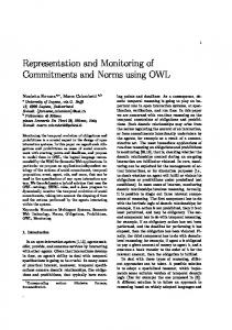
In this section, we give a complete statement of the used car buyer’s (UCB) problem [Howard 1962]. This problem is highly asymmetric. Howard [1962] describes a decision tree representation and solution of this problem. Smith, Holtzman and Matheson [1993] describe a representation and solution of this problem based on a generalization of the symmetric influence diagram technique [Howard and Matheson 1981, Olmsted 1983, Shachter 1986, Ezawa 1986, Tatman 1986]. A statement of the UCB problem is as follows. Joe is considering buying a used car from a dealer for $1,000. The market price of similar cars with no defects is $1,100. Joe is uncertain whether the particular car he is considering is a “peach” or a “lemon.” Of the ten major subsystems in the car, a peach has a serious defect in only one subsystem, whereas a lemon has a serious defect in six subsystems. The probability that the used car under consideration is a lemon is 0.2. The cost of repairing one defect is $40, and the cost of repairing six defects is $200. For an additional $60, Joe can buy the car from the dealer with an “anti-lemon guarantee.” The anti-lemon guarantee will normally pay for 50% of the repair cost, but if the car is a lemon, then the guarantee will pay 100% of the repair cost. Before buying the car, Joe has the option of having the car examined by a mechanic for an hour. In this time period, the mechanic offers three alternatives, t1, t2, and t3 as follows: t1: Test the steering subsystem alone at a cost of $9; t2: Test the fuel and electrical subsystems for a total cost of $13; t3: Do a two-test sequence in which Joe can authorize a second test after the result of the first test is known. In this alternative, the mechanic will first test the transmission subsystem at a cost of $10 and report the results to Joe. If Joe approves, the mechanic will then proceed to test the differential subsystem at an additional cost of $4. All tests are guaranteed to find a defect in the subsystems if a defect exists. We assume that Joe’s utility for profit is linear in dollars. A decision tree representation and solution of this problem is shown in Figures 1 and 2. Figure 1 shows the preprocessing of probabilities, and Figure 2 shows a decision tree representation and solution. The optimal strategy is to do test t2; if both systems are non-defective then buy with no guarantee, else buy with guarantee. The maximum expected utility is $32.87.

Prakash P. Shenoy

7

Figure 1. The preprocessing of probabilities in the UCB problem.

1/10 d1 0.80 p

0 d2

9/10

~d 2 1 1/9 d2

l 0.20

~d 2 8/9 5/9 d2 ~d 2 4/9 6/9 d2

4/10

~d 2 0.67

3/9

S l .05 0.40 0.60 .08 p

.64 R1

.07 0.17 d2 .05 .05

~d1 0.80

0.83 .03

S l .05 0.40 0.96 .64 p

R2

~d 2

R2

~d 2

l .07 1 0.60 .08 p

R2

R2

R1

~d 1

0.20 d1

.08

0

S

.08

R2

S 6/10 d1

0.33 d2

R2

R1

~d 1

0 p

0

S l .03 0.40


8

Figure 2. A decision tree representation and solution of the UCB problem. 28 S

p, 0.8

g 24 S

p, 0.8

b 28

nt, 0

B

l, 0.2

l, 0.2

60 –100 20 40

~b 0 –36 S

p, 0.4

g 32 S

p, 0.4

44 S

p, 0.9

g 22 S

p, 0.9

b 32

d1 , 0.20

B

l, 0.6

l, 0.6

60 –100 20 40

~b 0 t 1, –9

R1 41.60

l, 0.1

b 44 B ~d1 , 0.80

l, 0.1

60 –100 20 40

~b 0 –100 S

p, 0

g 40 S

p, 0

b 40

32.87

B T1 32

t 2 , –13

~d 2 , 0.67

R1

28 B

d2 , 0.17

–100 20 40 0

–4 S

p, 0.6

28 g S

p, 0.6

R2 b

45.87

l, 1

60

~b

d2 , 0.33 d1 , 0.20

l, 1

l, 0.4

l, 0.4

60 –100 20 40

~b 0

49.33 ~d1 , 0.80

53.60 p, 0.96

R2

S b ~d 2 , 0.83

53.60 B

g

l, 0.04

20.80 p, 0.96 S

l, 0.04

60 –100 20 40

~b 0 c, –4 d1 , 0.20

32 T2 s, 0

t 3 , –10

42.66 R1 c, –4 45.33 ~d1 , 0.80

T2 s, 0

Prakash P. Shenoy

3

9

VALUATION NETWORK REPRESENTATION

In this section, we describe the valuation network representation technique and illustrate it using the UCB problem. The representation technique described here is a generalization of the valuation network representation technique described in Shenoy [1992a, 1993] for symmetric decision problems. To deal with asymmetries in decision problems, we introduce the concepts of indicator valuations and effective frames. An indicator valuation is a special type of a probability valuation, and an effective frame is a subset of a frame. A valuation network representation is specified at three levels—graphical, dependence, and numeric. This is somewhat analogous to Howard and Matheson’s [1981] relational, functional, and numerical levels of specification in influence diagrams. The graphical and dependence levels have qualitative (or symbolic) knowledge, whereas the numeric level has quantitative knowledge. Figure 3. A valuation network for the UCB problem.

ι1

ρ1

ι2

ρ2

T1

R1

T2

R2

υ1

υ2

σ

B

S

υ3

3 . 1 Graphical Level At the graphical level, a valuation network representation consists of a graph called a valuation network. Figure 3 shows a valuation network for the UCB problem. A valuation network consists of two types of nodes—variable and valuation. Variables are further classified as either decision or chance, and valuations are further classified as either indicator, or probability, or utility. Thus in a valuation network, there are five different types of nodes—decision, chance, indicator, probability, and utility. Using knowledge-based systems terminology, the collection of decision and chance variables constitute a description of the problem at the propositional level, and the collection of indicator, probability, and utility valuations constitute a description of the problem at the knowledge level. Decision Nodes. Decision nodes correspond to decision variables and are depicted by rectangles. In the UCB problem, there are three decision nodes labeled T1, T2, and B. T1 represents


10

the first test decision, T2 represents the second test decision, and B represents the buy car decision. The values of the decision variables (i.e., the alternatives) are not shown in the valuation network. The set of values of a variable is called the frame for that variable. The frames of decision variables are specified at the dependence level description of the valuation network representation (in Subsection 3.2). Chance Nodes. Chance nodes correspond to chance variables and are depicted by circles. In the UCB problem, there are three chance nodes labeled R1, R2, and S. R1 represents the first test results, R2 represents the second test results, and S represents the state of the car. As in the case of decision variables, the values of chance variables are not shown in the valuation network. The frames of chance variables are specified in the dependence level description of the valuation network representation (in Subsection 3.2). Let -D denote the set of all decision variables, let -R denote the set of all chance variables, and let - = -D∪-R denote the set of all variables. In this paper we are concerned only with the case where - is finite. We use upper-case Roman alphabets to denote variables. Indicator Valuations. Indicator valuations represent qualitative constraints on the joint frames of decision and chance variables and are depicted by double-triangular nodes. The set of variables directly connected to an indicator valuation by undirected edges constitutes the domain of the indicator valuation. In the UCB problem, there are two indicator valuations labeled ι1 and ι2. ι1’s domain is {T1, R1}, and ι2’s domain is {T1, T2, R2}. ι1 represents the constraint that first test result is not available if Joe decides not to do any of three tests proposed by the mechanic at T1. ι2 represents the constraints that at T2, the option to stop or continue is available only if Joe decides on test t3 proposed by the mechanic at T1, and that the second test result is available only if Joe decides on test t2 at T1, or if he decides on test t3 at T1 and decides to continue at T2. The details of the indicator valuations are specified at the dependence level description of the valuation network representation (in Subsection 3.2). Utility Valuations. Utility valuations represent factors of the joint utility function and are depicted by diamond-shaped nodes in valuation networks. The set of variables directly connected to a utility valuation constitutes the domain of the utility valuation. Depending on whether the utility function decomposes additively or multiplicatively, the factors are additive or multiplicative (or perhaps some combination of the two). In the UCB problem, there are three additive utility valuations labeled υ1, υ2, and υ3. υ1’s domain is {T1}, υ2’s domain is {T2}, and υ3’s domain is {B, S}. υ1 represents the cost of the first test, υ2 represents the cost of the second test, and υ3 represents the value of the car less the cost of buying the car and repairing the defects. The details of the utility valuations are specified at the numeric level description of the valuation network representation (in Subsection 3.3). Probability Valuations. Probability valuations represent multiplicative factors of the family of joint probability distributions of the chance variables in the problem, and are depicted by triangular nodes in valuation networks. The set of all variables directly connected to a probability val-

Prakash P. Shenoy

11

uation constitutes the domain of the probability valuation. If a probability valuation is a conditional, then this is indicated by making the edges between the probability valuation node and the variables in the head of the conditional directed toward the variables. In the UCB problem, there are three probability valuations labeled σ, ρ1, and ρ2. σ’s domain is {S}, ρ1’s domain is {R1, S}, and ρ2’s domain is {R1, R2, S}. The arrow from σ to S indicates that σ is a conditional for {S} given ∅. The details of the probability valuations are specified at the numeric level description of the valuation network representation (in Subsection 3.3). The precise meaning of the probability valuations is given in Subsection 3.3 and Subsection 4.2. Information Constraints. The specification of the valuation network at the graphical level includes directed arcs between pairs of distinct variables. These directed arcs represent information constraints. Suppose R is a chance variable and suppose D is a decision variable. An arc R→D means that the true value of R is known to the decision maker (DM) when the DM chooses an alternative from D’s frame, and an arc from D→R means that the true value of R is not known to the DM at the time the DM has to choose an alternative from D’s frame. Well-Defined Information Constraints. We say the information constraints are welldefined if they satisfy the following condition: For any chance variable R and for any decision variable D, either there is a directed path from R to D, or there is a directed path from D to R, but not both. (We say there is a directed path from X to Y if either X→Y or there exists Z1, ..., Zk for some k ≥ 1 such that X→Z1, Z1→Z2, ..., Zk–1→Zk, Zk→Y.) The rationale behind the definition of well-defined information constraints is as follows. The information constraints are used during the solution phase to solve the valuation network representation. The information constraints dictate what deletion sequences are valid for deleting variables during the solution phase. If there is a directed path from D to R, then R must be deleted before D, and if there is a directed path from R to D, then D must be deleted before R. If there is neither a directed path from D to R nor a directed path from R to D, then depending on whether R is deleted before D or not, we may get different solutions to the decision problem. On the other hand, if there is a directed path from D to R and a directed path from R to D, then there does not exist a valid deletion sequence, and we are unable to solve the problem. We assume that the DM has perfect recall. This means that if there is a directed path from R to D, then the DM knows the true value of R at the time the DM has to choose an alternative from D’s frame, and if there is a directed path from D to R, then this means that the DM does not know the true value of R at the time the DM has to choose an alternative from D’s frame. In the UCB problem, for example, at the time Joe makes a buy decision, he knows the results of the first test and the second test, but not the state of the car. If the information constraints are well-defined, then given any chance variable R and any decision variable D, either the DM knows the true value of R (at the time the DM has to choose an alternative from D’s frame) or not. If the information constraints are not well-defined, then this means that either the information constraints are incompletely specified or that the information constraints are contradictory.


12

3 . 2 Dependence Level Next, we specify valuation network representation at the dependence level. Like the graphical level, specification of a valuation network representation at the dependence level involves only qualitative (or symbolic) knowledge. In this sense, the dependence level of a valuation network representation is different from the function level of influence diagram representation since the latter may involve arithmetic operations. Frames. Associated with each variable X is a frame 0X. We assume that all variables have finite frames. The frame of a decision variable consists of alternatives available to the DM. The frame of a chance variable consists of all mutually exclusive and exhaustive values that the chance variable can assume. We use the terminology “frame” (as opposed to “sample space”) to emphasize the fact that the possibilities that comprise a frame are neither determined nor meaningful independent of our knowledge [Shafer 1976, p. 36]. In the UCB problem, 0T1 = {nt, t1, t2, t3}, where nt denotes no test, and ti denotes the ith test option offered by the mechanic, i = 1, 2, and 3; 0R1 = {n1, d1, ~d1}, where n1 denotes no result, d1 denotes the first subsystem tested is defective, and ~d1 denotes the first subsystem tested is non-defective; 0T2 = {nc, s, c}, where nc denotes no choice, s denotes stop, and c denotes continue; 0R2 = {n2, d2, ~d2}, where n2 denotes no result, d2 denotes the second subsystem tested is defective, and ~d2 denotes the second subsystem tested is non-defective; 0B = {b, g, ~b}, where b denotes buy with no guarantee, g denotes buy with guarantee, and ~b denotes do not buy; and 0S = {p, l} where p denotes the car is a peach, and l denotes the car is a lemon. Configurations. We often deal with non-empty subsets of variables in -. Given a nonempty subset h of -, let 0h denote the Cartesian product of 0X for X in h, i.e., 0h = ×{0X | X ∈ h}. We can think of 0h as the set of possible values of the joint variable h. Accordingly, we call 0h the frame for h. Also, we refer to elements of 0h as configurations of h. We use this terminology even when h consists of a single variable, say X. Thus we refer to elements of 0X as configurations of X. We use lower-case, bold-faced letters such as x, y, etc., to denote configurations. Also, if x is a configuration of g, y is a configuration of h, and g∩h = ∅, then (x, y) denotes a configuration of g∪h. It is convenient to extend this terminology to the case where the set of variables h is empty. We adopt the convention that the frame for the empty set ∅ consists of a single configuration, and we use the symbol ♦ to name that configuration; 0∅ = {♦}. To be consistent with our notation above, we adopt the convention that if x is a configuration, then (x,♦) = x. Indicator Valuations. Earlier we described indicator valuations as qualitative constraints on the joint frames of variables. Here, we define them formally. Suppose s is a subset of variables. An indicator valuation for s is a function ι: 0s → {0, 1}. The only values assumed by an indicator valuation are 0 and 1, hence the term indicator valuation. The values of indicator valuations can be treated as (degenerate) probabilities. An efficient way of representing an indicator valuation is

Prakash P. Shenoy

13

simply to describe the elements of the frame that have value 1, i.e., we represent ι by Ωι where Ωι = {x ∈ 0s | ι(x) = 1}. Obviously, Ωι ⊆ 0s. To minimize jargon, we also call Ωι an indicator valuation for s. In the UCB problem, we have two indicator valuations—ι1 (or Ωι ) with domain {T1, R1}, 1

and ι2 (or Ωι2) with domain {T1, T2, R2}. These indicator valuations are specified as follows: Ω ι = {(nt, n1), (t1, d1), (t1, ~d1), (t2, d1), (t2, ~d1), (t3, d1), (t3, ~d1)}; 1 and Ω ι = { (nt, nc, n2), (t1, nc, n2), (t2, nc, d2), (t2, nc, ~d2), (t3, s, n2), (t3, c, d2), (t3, c, ~d2)} . 2

ι1 represents the constraint that the first test result is not available if Joe decides not to do any of the three tests proposed by the mechanic at T1. ι2 represents the constraints that at T2, the option to stop or continue is available only if Joe decides on test t3 proposed by the mechanic at T1, and that the second test result is available only if Joe decides on test t2 at T1, or if he decides on test t3 at T1 and decides to continue at T2. Figure 4 depicts the two indicator valuations graphically. Figure 4. A graphical depiction of Ωι1 and Ωι2. Ωι nt

Ωι

1

R1

n1

nt

d1 t1

R1 d1

T1

t2

T2

R1

nc

nc

s ~d1 d1

t3

T2

nc

R2 R2

n2 n2 d2

~d1

T1 t2

t1

T2

2

t3

~d1

R2

~d2 n2 d2

T2 c

R1

R2

R2 ~d2

Some indicator valuations constrain domains of chance variables. For example, ι1 constrains the domain of R1. Some indicator valuations constrain domains of decision variable. And some indicator valuations constrain the domains of both decision and chance variables. For example ι2 constrains the domains of T2 and R2. The concept of indicator valuations is crucial to the computational efficiency of the solution technique. Using the indicator valuations in a problem, we define the “effective frame” for a subset


14

of variables. The effective frame for s is a subset of the frame for s. The increased computational efficiency of the solution technique is partly the result of working on effective frames instead of working on frames. In the remainder of this subsection, we introduce some notation and definitions to enable us to define the effective frame for a subset of variables. Projection of Configurations. Projection of configurations simply means dropping extra coordinates; if (t3, d1, c, ~d2) is a configuration of {T1, R1, T2, R2}, for example, then the projection of (t3, d1, c, ~d2) to {T1, R1} is simply (t3, d1), which is a configuration of {T1, R1}. If g and h are sets of variables, h ⊆ g, and x is a configuration of g, then let x↓h denote the projection of x to h. The projection x↓h is always a configuration of h. If h = g and x is a configuration of g, then x↓h = x. If h = ∅, then x↓h = ♦. Marginalization of Indicator Valuations. Suppose Ωιa is an indicator valuation for a, and suppose b ⊆ a. The marginalization of Ωιa to b, denoted by Ωιa↓b, is an indicator valuation for b given by Ω ιa↓b = {x ∈ 0 b | (x, y) ∈ Ω ι for some y ∈ 0 a–b}. a

To illustrate this definition, consider the indicator valuation Ωι2 for {T1, T2, R2} in the UCB problem. The marginal of Ωι2 for {T1, T2} is given by the indicator valuation Ω ι2↓{T1, T2} = {(nt, nc), (t1, nc), (t2, nc), (t3, s), (t3, c)}.

Combination of Indicator Valuations. Suppose Ωι is an indicator valuation for a, and a suppose Ωιb is an indicator valuation for b. The combination of Ωιa and Ωιb, denoted by Ωιa⊗Ωιb, is an indicator valuation for a∪b given by Ω ιa⊗Ω ιb = {x ∈ 0 a∪b | x

↓a

∈ Ω ιa and x

↓b

∈ Ω ιb}.

To illustrate this definition, consider the two indicator valuations Ωι1 and Ωι2 in the UCB problem. The combination Ωι ⊗Ωι is an indicator valuation for {T1, R1, T2, R2} given as fol1 2 lows: Ω ι ⊗Ω ι = { (nt, n1, nc, n2), (t1, d1, nc, n2), (t1, ~d1, nc, n2), (t2, d1, nc, d2), 1

2

(t2, d 1, nc, ~d 2), (t2, ~d 1, nc, d 2), (t2, ~d 1, nc, ~d 2), (t3, d 1, s, n 2), (t3, d 1, c, d 2), (t3, d 1, c, ~d 2), (t3, ~d 1, s, n 2), (t3, ~d 1, c, d 2), (t3, ~d 1, c, ~d 2)} . Effective Frames. Suppose {Ωι1, ..., Ωιp} is the set of indicator valuations in a given problem such that Ωιj is an indicator valuation for sj, j = 1, ..., p. Without loss of generality, assume that s1∪...∪sp = -. (If a variable, say X, is not included in the domain of some indicator valuation, include the vacuous indicator valuation Ωι for {X}, i.e., Ωι = 0X.) Suppose s is a subset of variables. The effective frame for s, denoted by Ωs, is given by Ω s = (⊗{Ω ιk | sk∩s ≠ ∅})↓s. In words, the effective frame for s is defined in two steps as follows. First we combine indicator valuations whose domains include a variable in s. Second, we marginalize the resulting combination to eliminate variables not in s.

Prakash P. Shenoy

15

To illustrate this definition, consider the indicator valuations Ωι1 for {T1, R1}, and Ωι2 for {T1, T2, R2}. Since B and S are not included in the domains of the two indicator valuations, we need to introduce vacuous indicator valuations Ωι for {B} and Ωι for {S}. Then, for example, 3 4 the effective frame for {R1, R2, S} is given by Ω{R , R , S} = (Ωι ⊗Ωι ⊗Ωι )↓{R1, R2, S} 1

2

1

2

4

= { (n 1, n 2, p), (n 1, n 2, l), (d 1, n 2, p), (d 1, n 2, l), (d 1, d 2, p), (d 1, d 2, l), (d 1, ~d 2, p), (d1, ~d2, l), (~d1, n2, p), (~d1, n2, l), (~d1, d2, p), (~d1, d2, l), (~d1, ~d2, p), (~d1, ~d2, l)}. As we will see shortly, all the numeric information in probability and utility valuations are specified on effective frames only. Also, in the solution phase, all numerical computations are done on effective frames. The definitions of marginalization and combination of indicator valuations allow us to define effective frames in terms of indicator valuations. In Section 5, we describe an efficient method to compute effective frames using local computation. 3.3

Numeric Level

Finally, we specify a valuation network at the numeric level. At this level, we specify the details of the utility and probability valuations. Utility Valuations. Suppose u ⊆ -. A utility valuation υ for u is a function υ: Ωu → R, where R is the set of real numbers. The values of υ are utilities. If υ is a utility valuation for u, we say u is the domain of υ. In the UCB problem, there are three utility valuations υ1 for {T1}, υ2 for {T2}, and υ3 for {B, S}. Table I shows the details of these utility valuations. Table I. Utility valuations in the UCB problem. ΩT

υ1

ΩT

υ2

Ω{B, S}

nt t1 t2 t3

0 –9 –13 –10

nc c s

0 –4 0

b p b l g p g l ~b p ~b l

1

2

υ3 60 –100 20 40 0 0

What are the semantics of utility valuations? Each utility valuation is a “factor” of the joint utility valuation. Naturally, we need to specify how the utility valuations combine to define the joint utility valuation. In the UCB problem, the utility valuations combine by pointwise addition. A formal definition is as follows. Combination of Utility Valuations. Suppose h and g are subsets of -, suppose υi is a utility valuation for h, and suppose υj is a utility valuation for g. Then the combination of υi and υj, denoted by υi⊗υj, is a utility valuation for h∪g defined as follows:


16

(υ i⊗υ j)(x) = υ i(x ↓h) + υ j(x ↓g) for all x ∈ Ωh∪g. Thus combination of utility valuations is pointwise addition. This definition assumes of course that υi and υj are additive factors of υi⊗υj. (If υi and υj were multiplicative factors, we would have defined combination as pointwise multiplication.) In the UCB problem, the joint utility function is given by the utility valuation υ1⊗υ2⊗υ3 for {T1, T2, B, S}. As we will see, it is not necessary to compute the joint utility valuation to solve a decision problem. The only reason for defining the joint utility valuation is to explain what each utility valuation represents, namely a factor of the joint. Probability Valuations. Suppose r ⊆ -. A probability valuation ρ for r is a function ρ: Ωr → [0, 1]. The values of ρ are probabilities. If ρ is a valuation for r, then we say r is the domain of ρ. In the UCB problem, there are three probability valuations, σ for {S}, ρ1 for {S, R1}, and ρ2 for {S, R1, R2}. Table II shows the details of these probability valuations. What are the semantics of probability valuations? In general, each probability valuation is a factor of the joint probability valuation. Naturally, we need to specify how the probability valuations combine to define the joint probability valuation. Also, to define conditionals—a special type of a probability valuation—we need to define marginalization of probability valuations and division for probability valuations. After we define these terms, we will explain precisely what the three probability valuations in the UCB problem mean. Combination of Probability Valuations. Probability theory defines combination as an operation that combines probability valuations by pointwise multiplication. A formal definition is as follows. Suppose h and g are subsets of -, suppose ρi is a probability valuation for h, and suppose ρj is a probability valuation for g. Then the combination of ρi and ρj, denoted by ρi⊗ρj or ρj⊗ρi), is a probability valuation for h∪g such that (ρ i⊗ρ j)(x) = (ρ j⊗ρ i)(x) = ρ i(x ↓h) ρ j(x ↓g) for all x ∈ Ωh∪g. Marginalization of Probability Valuations. Probability theory defines marginalization as an operation that reduces the domain of a probability function. Suppose h is a subset of containing (chance or decision) variable X, and suppose ρ is a probability valuation for h. The marginal of ρ for h − {X}, denoted by ρ↓(h − {X}), is a probability valuation for h − {X} such that ρ↓(h − {X})(c) = Σ {ρ(c, x)| x ∈ 0 X ∋ (c, x) ∈ Ω h} for all c ∈ Ωh − {X}. Suppose ρ is a probability valuation for r. We say ρ is a probability distribution for r if and only if ρ↓∅(♦) = 1, i.e., if the values of ρ sum to 1. Division. Finally, probability theory defines a division operation (for defining conditionals). Suppose α is a probability valuation for g, and suppose h ⊆ g. Then we define α/α↓h, called α divided by α↓h, to be a probability valuation for g defined as follows:

Prakash P. Shenoy

17

(α/α↓h)(r) = α(r)/α↓h(r↓h) for all r ∈ Ωg. If α(r) = α↓h(r↓h) = 0, then we consider (α/α↓h)(r) = 0. In all other respects, the division in the right hand side of the definition above should be interpreted as the usual division of ↓h ↓h two real numbers. Since α (r↓h) ≥ α(r) ≥ 0 for all r ∈Ωg, the values of α/α lie in the interval [0, 1]. Table II. Probability valuations in the UCB problem. ΩS

σ

p l

.80 .20

Ω{S, R } 1

p p p l l l

n1 d1 ~d1 n1 d1 ~d1

ρ1 1 1/10 9/10 1 6/10 4/10

Ω{S, R p p p p p p p l l l l l l l

1,

n1 d1 ~d1 d1 d1 ~d1 ~d1 n1 d1 ~d1 d1 d1 ~d1 ~d1

R 2}

n2 n2 n2 d2 ~d2 d2 ~d2 n2 n2 n2 d2 ~d2 d2 ~d2

ρ2 1 1 1 0/9 9/9 1/9 8/9 1 1 1 5/9 4/9 6/9 3/9

Conditionals. Suppose α is a probability distribution for a∪b, where a and b are disjoint subsets of variables. We call χ = α/α↓b a conditional for a given b. We call a the head of (the domain of) χ, and we call b the tail of χ. Suppose χ = α/α↓b is a conditional for a given b. Then it is easy to see that χ↓b is an identity for α, i.e., α⊗χ↓b = α. Also, it is easy to see that χ/χ↓b = χ. We will exploit these properties of conditionals to avoid unnecessary division operations in the fusion algorithm. If a probability valuation is a conditional by itself, then this is specified in the valuation network by directing the edges between a conditional and its head toward the head. In the UCB problem, for example, σ is a conditional for {S} given ∅. Combination of an Indicator and a Probability Valuation. Suppose h and g are subsets of -, suppose ι is an indicator valuation for h, and suppose ρ is a probability valuation for g. Then the combination of ι and ρ, denoted by ι⊗ρ or ρ⊗ι, is a probability valuation for h∪g defined as follows: (ι⊗ρ)(x) = (ρ⊗ι)(x) = ρ(x↓g) for all x ∈ Ωh∪g. In combining an indicator valuation and a probability valuation, there is no computation involved since the values of an indicator valuation are identically one over the effective


18

frame. However, indicator valuations do contribute domain information to the combination, i.e., the domain of ι⊗ρ is h∪g whereas the domain of ρ is g. Table III. The conditionals in the UCB problem. Ω{S, T1, R1} p p p p p p p l l l l l l l

nt t1 t1 t2 t2 t3 t3 nt t1 t1 t2 t2 t3 t3

n1 d1 ~d1 d1 ~d1 d1 ~d1 n1 d1 ~d1 d1 ~d1 d1 ~d1

ρ 1⊗ι 1 1 1/10 9/10 1/10 9/10 1/10 9/10 1 6/10 4/10 6/10 4/10 6/10 4/10

Ω{S, T1, R1, T2, R2} p p p p p p p p p p p l l l l l l l l l l l

nt t1 t1 t2 t2 t3 t3 t3 t3 t3 t3 nt t1 t1 t2 t2 t3 t3 t3 t3 t3 t3

n1 d1 ~d1 d1 ~d1 d1 d1 d1 ~d1 ~d1 ~d1 n1 d1 ~d1 d1 ~d1 d1 d1 d1 ~d1 ~d1 ~d1

nc nc nc nc nc c c s c c s nc nc nc nc nc c c s c c s

ρ 2⊗ι 2 n2 n2 n2 n2 n2 d2 ~d2 n2 d2 ~d2 n2 n2 n2 n2 n2 n2 d2 ~d2 n2 d2 ~d2 n2

1 1 1 1 1 0/9 9/9 1 1/9 8/9 1 1 1 1 1 1 5/9 4/9 1 6/9 3/9 1

Semantics of Probability Valuations in the UCB Problem. In the UCB problem, the probability valuation σ for {S} is the marginal for S. The probability valuation ρ1⊗ι1 for {T1, R1, S} is a conditional for {R1} given {S, T1} (see Table III). The values of this conditional are specified implicitly in the statement of the problem. The conditional for {R1} given {S, T1} factors into ρ1 and ι1. ρ1 contains the numeric information of this conditional, and ι1 contains the structural information of this conditional. ρ1 can be given precise semantics as follows. For x ∈ Ω{R1, S}, ρ1(x) represents the conditional probability of x↓R1 given x↓S and the fact that x is not ruled out by structural constraints. For example, ρ1(p, n1) = 1 because since no result (n1) is not ruled out by structural constraints, and it is the only value of R1 possible in this circumstance, its conditional probability must be 1. The probability valuation ρ2⊗ι2 for {T1, R1, T2, R2, S} is a conditional for {R2} given {S, T1, R1, T2} (see Table III). The values of this conditional are specified implicitly in the problem

Prakash P. Shenoy

19

statement. As in the previous case, this conditional factors into ρ2 and ι2. Also, using the same ↓R ↓{S, R1} argument as in the case of σ, ρ2(x) represents the conditional probability of x 2 given x ↓R and the fact that x 2 is not ruled out by structural constraints. Summary. We have now completely defined a valuation network representation of a decision problem. In summary, a valuation network representation of a decision problem ∆ consists of decision variables, chance variables, indicator valuations, probability valuations, utility valuations, and information constraints, ∆ = { - D , - R , { ι1, ..., ιp} , { υ 1, ..., υ m } , { ρ 1, ..., ρ n} , → } . In the next section, we describe the meaning and solution of a valuation network representation. 4 SEMANTICS & SOLUTION OF A VALUATION NETWORK REPRESENTATION The main goal of this section is to explain the meaning of utility valuations, indicator valuations, and probability valuations. This will enable us to define when a valuation network representation is well-defined, and what it means to solve a well-defined valuation network representation. Although most of this material is stated in [Shenoy 1992a], there are two points of departure. First we need to account for indicator valuations. Second, the definition of a well-defined valuation network representation stated here is weaker than the corresponding definition in [Shenoy 1992a]. This has an important implication in the solution technique. This section is organized into two subsections. In Subsection 4.1, we define the concept of a canonical valuation network. In Subsection 4.2, we use the concept of a canonical valuation network to define what it means for a valuation network representation to be well-defined and to define what it means to solve a valuation network representation. 4 . 1 A Canonical Valuation Network Representation A canonical valuation network ∆C = {{D}, {R}, {υ}, {ρ}, →} consists of a decision variable D with a finite frame 0D, a chance variable R with a finite frame 0R, a utility valuation υ for {D, R}, a conditional ρ for {R} given {D}, and a precedence relation → defined by D→R. Figure 5 shows a canonical valuation network and an equivalent decision tree representation. The meaning of the canonical valuation network is as follows. The elements of 0D are alternatives, and the elements of 0R are states of nature. The conditional ρ for {R} given {D} is a family of probability distributions for R, one for each alternative d ∈ 0D. In other words, the probability distribution of chance variable R is conditioned on the alternative d chosen by the decision maker. The probability ρ(d, r) can be interpreted as the conditional probability of R = r given D = d. Since ρ is a conditional for {R} given {D}, it follows that ρ↓{D}(d) = 1 for all d ∈ 0D.

(4.1)

The utility valuation υ is a conditional utility function—if the decision maker chooses alternative d and the state of nature r prevails, then the utility to the decision maker is υ(d, r). The precedence


20

relation → states that the true state of nature is revealed to the decision maker only after the decision maker has chosen an alternative. Figure 5. A canonical valuation network and an equivalent decision tree representation. ρ(d1 , r 1 ) r1 ρ d1 R

D

υ

D

R

. . .

. . .

rm ρ(d1 , r m) ρ(dn , r 1 ) r1

dn R

. . .

rm ρ(dn , r m)

υ(d1 , r 1 )

υ(d1 , r m) υ(dn , r 1 )

υ(dn , r m)

Before we can describe how to solve a canonical decision problem, we need some definitions. We give formal definitions for combining a probability and a utility valuation, marginalizing a chance variable out of the domain of a utility valuation, marginalizing a decision variable out of the domain of a utility valuation, and defining a decision function associated with marginalizing a decision variable out of the domain of a utility valuation. Combination of a Utility and a Probability Valuation. In the previous section, we defined combination of two utility valuations, and combination of two probability valuations. Here we define combination of a utility and a probability valuation, and combination of a utility and an indicator valuation. Suppose h and g are subsets of -, suppose υ is a utility valuation for h, and suppose ρ is a probability valuation for g. Then the combination of υ and ρ, denoted by υ⊗ρ (or ρ⊗υ), is a utility valuation for h∪g defined as follows: (υ⊗ρ)(x) = (ρ⊗υ)(x) = υ(x↓h) ρ(x↓g)

(4.2)

for all x ∈ Ωh∪g. Combination of a Utility and an Indicator Valuation. Suppose h and g are subsets of -, suppose υ is a utility valuation for h, and suppose ι is an indicator valuation for g. Then the combination of υ and ι, denoted by υ⊗ι (or ι⊗υ), is a utility valuation for h∪g defined as follows: (υ⊗ι)(x) = (ι⊗υ)(x) = υ(x↓h) for all x ∈ Ωh∪g. In combining an indicator valuation and a utility valuation, there is no computation involved (since the values of an indicator valuation are identically one over the

(4.3)

Prakash P. Shenoy

21

effective frame). However, indicator valuations do contribute domain information to the combination, i.e., the domain of υ⊗ι is h∪g whereas the domain of υ is h. Marginalization of Utility Valuations. In the previous section, we defined marginalization for probability valuation. Here we define marginalization for utility valuations. The definition of marginalization of utility valuations depends on the nature of the variable being deleted. Suppose h is a subset of - containing chance variable R, and suppose α is a utility valuation for h. The marginal of α for h−{R}, denoted by α↓(h−{R}), is a utility valuation for h−{R} defined as follows: α↓(h−{R})(c) = Σ {α(c, r)| r ∈ ΩR ∋ (c, r) ∈ Ωh}

(4.4)

for all c ∈ Ωh−{R}. Suppose h is a subset of - containing decision variable D, and suppose α is a utility valuation ↓(h−{D})

for h. The marginal of α for h−{D}, denoted by α as follows:

, is a utility valuation for h−{D} defined

α↓(h−{D})(c) = MAX{α(c, d)| d ∈ ΩD ∋ (c, d) ∈ Ωh}

(4.5)

for all c ∈ Ωh−{D}. Decision Functions. Each time we marginalize a decision variable D from a utility valuation α for h, we implicitly determine a decision function. Suppose α is a utility valuation for h, and suppose D is a decision variable in h. A decision function for D with respect to α is a function ξD: Ωh–{D} → ΩD such that ξD(c) = d whenever α↓h−{D}(c) = α(c, d). Intuitively, a decision function is rule for selecting an alternative d from the frame of D on the basis of the information c about chance and decisions variables in h–{D}. A decision function ξD: Ωh–{D} → ΩD can be encoded as an indicator valuation ζD for h as follows: ζD(c, d) =

1  0

if ξD(c) = d (4.6)

otherwise for all (c, d) ∈ Ωh. We also call indicator valuation ζD a decision function for D with respect to α. Strategy. A strategy σ is a collection of decision functions, one for each decision variable in -D, i.e., σ = {ξD}D ∈ -D. In the canonical valuation network, since there is only one decision variable, a strategy is simply one decision function. Also, since the true value of R is not known when decision D is made, a decision function for D, ξD: Ω∅ → ΩD, is simply a configuration d = ξD(♦) in ΩD. Suppose σ = {ξD}D ∈ -D is a strategy, and suppose y is a configuration of -R. Then σ and y together determine a unique configuration of -D. Let aσ,y denote this unique configuration of -D. By definition, aσ,y↓{D} = ξD(y↓h–{D}), where h is the domain of the valuation α with respect to which ξD is defined.


22

Valid Deletion Sequences. Suppose → is a binary relation on - representing well-defined information constraints. Suppose g = {X1, ..., Xk} is a subset of -. We call X1 a minimal variable of g if there does not exist Xj ∈ g such that X1→Xj. We call X1X2...Xk a valid deletion sequence of variables in g if and only if X1 is a minimal variable in g, X2 is a minimal variable in g−{X1}, ..., and Xk–1 is a minimal variable in g–{X1, ..., Xk–2}. Marginalizing a Subset of Variables from Utility Valuations. Suppose h and g are non-empty subsets of - such that g is a proper subset of h, suppose α is a utility valuation for h, and suppose → is a binary relation on - representing well-defined information constraints. The ↓g

marginal of α for g with respect to the binary relation →, denoted by α , is a valuation for g defined as follows: α ↓g = ( ( (α ↓(h−{X 1 }) ) ↓(h−{X 1 , X 2 }) ) ...) ↓(h−{X 1 , X 2 , ..., Xk })

(4.7)

where h−g = {X1, ..., Xk}, and X1X2...Xk is a valid deletion sequence of variables in h−g. Solving a Canonical Valuation Network. Solving a canonical valuation network using the criterion of maximizing expected utility is easy. Informally, first, we combine ρ and υ by pointwise multiplication. The result is a utility valuation ρ⊗υ for {D, R}. Next we marginalize R out of ρ⊗υ using addition. The result is a utility valuation (ρ⊗υ)↓{D} for {D}. Each value ↓{D}

(ρ⊗υ) (d) represents expected utility if alternative d is chosen by the DM. Next, we marginalize D out of (ρ⊗υ)↓{D} using maximization. The result is a utility valuation ((ρ⊗υ)↓{D})↓∅ for ∅. The value ((ρ⊗υ)↓{D})↓∅(♦) is the maximum expected utility, and an optimal alternative is d* ∈ 0D such that (ρ⊗υ)↓{D}(d*) = ((ρ⊗υ)↓{D})↓∅(♦). Notice that we marginalize R before D. This is a consequence of the precedence relation D→R. If the DM had perfect information, then this would be represented in the canonical valuation network by the precedence relation R→D, and in this case, we would marginalize D before R, and the maximum expected utility is ((ρ⊗υ)↓{R})↓∅(♦). The difference ↓{R} ↓∅

↓{D} ↓∅

((ρ⊗υ) ) (♦) − ((ρ⊗υ) ) (♦) is called the expected value of perfect information. In summary, the maximum expected utility associated with an optimal alternative is (ρ⊗υ)↓∅(♦), and alternative d* is optimal if and only if (ρ⊗υ)↓{D}(d*) = (ρ⊗υ)↓∅(♦). 4.2

Well-Defined Valuation Network Representations

Consider a valuation network representation of a decision problem, ∆ = {-D, -R, {ι1, ..., ιp}, {υ1, ..., υm}, {ρ1, ..., ρn}, → }. We explain the meaning of ∆ by reducing it to an equivalent canonical valuation network ∆C = {{D}, {R}, {υ}, {ρ}, →}. To define ∆C, we need to define 0D, 0R, υ, and ρ. Define 0D such that for each distinct strategy σ of ∆, there is a corresponding alternative dσ in 0D. Define 0R such that for each distinct configuration y ∈Ω-R in ∆, there is a corresponding configuration ry in 0R. Before we define utility valuation υ for {D, R}, we need some notation. Consider the joint utility valuation υ1⊗...⊗υm in ∆. For convenience of exposition, suppose that the domain of this

Prakash P. Shenoy

23

utility valuation includes all of -D (if not, we can always vacuously extend it so it does). Typically the domain of this valuation also includes some (or all) chance variables. Let v denote the subset of chance variables included in the domain of the joint utility valuation, i.e., v ⊆ -R such that υ1⊗...⊗υm is a utility valuation for -D∪v. Define utility valuation υ for {D, R} such that υ(d σ , r y) = ( υ 1⊗...⊗υ m ) (a σ,y, y ↓v)

(4.8)

for all strategy σ of ∆, and for all configuration y ∈ Ω- . Remember that aσ,y is the unique conR figuration of -D determined by σ and y (see Subsection 4.1). Well-Defined Probability Valuations. Consider the joint probability valuation ι1⊗...⊗ιp⊗ρ1⊗...⊗ρn. For convenience of exposition, suppose that the domain of this probability valuation includes all of -R (if not, we can always vacuously extend it so it does). Let q denote the subset of decision variables included in the domain of the joint probability valuation, i.e., q ⊆ -D such that ι1⊗...⊗ιp⊗ρ1⊗...⊗ρn is a probability valuation for q∪-R. Note that q could be empty. Define probability valuation ρ for {D, R} such that ρ(d σ , r y ) = ( ι 1 ⊗...⊗ι p ⊗ρ 1 ⊗...⊗ρ n ) (a σ,y ↓q , y)

(4.9)

for all strategies σ, and for all configurations y ∈ Ω-R. ρ is a conditional if it satisfies condition (4.1). This motivates the following definition. We say {ι1, ..., ιp, ρ1, ..., ρn} is well-defined in ∆ if and only if

Σ { (ι1⊗...⊗ι p⊗ρ 1⊗...⊗ρ n)(a σ,y↓q, y) | y ∈ Ω - R} = 1

(4.10)

for each strategy σ. In general, checking whether or not a set of indicator and probability valuations are well defined is computationally intensive since we need to verify (4.10) for each strategy σ, and there are an exponential number of strategies. This is the case in the UCB problem, in which we have 63 distinct strategies. However, if a decision problem is in Howard canonical form [Howard 1990], i.e., none of the indicator valuations or probability valuations include a decision variable in their domains (i.e., q = ∅), then (4.10) reduces to simply checking whether ι1⊗...⊗ιp⊗ρ1⊗...⊗ρn is a probability distribution, and there are efficient methods that employ local computation to do this (e.g., [Shenoy 1992b]). Well-Defined Valuation Network Representation. Suppose ∆ = { - D , - R , { ι 1 , ...,

ιp}, {υ1, ..., υm}, {ρ1, ..., ρn}, → } is a decision problem. We say ∆ is well-defined if and only if {ι1, ..., ιp, ρ1, ..., ρn} is well-defined, and → is well-defined (see Subsection 3.1 for what it means for → to be well-defined).

In summary, in a valuation network representation ∆ of a decision problem, the utility valuations {υ1, ..., υm} represent the factors of a joint utility function υ, and the indicator and probability valuations {ι1, ..., ιp, ρ1, ..., ρn} represent the factors of a family of joint probability distributions ρ. Solving a Decision Problem. Suppose ∆ = { - D , - R , { ι 1 , ..., ι p } , { υ 1 , ..., υ m } , { ρ 1 , ..., ρn}, →} is a well-defined valuation network representation of a decision problem. Let ∆C =


24

{{D}, {R}, {υ}, {ρ}, →} denote the equivalent canonical valuation network representation. In the canonical valuation network ∆C, the two computations that are of interest are (1) the computa↓∅ tion of the maximum expected value (ρ⊗υ) (♦); and (2) the computation of an optimal alternative dσ* such that (ρ⊗υ)↓{D}(dσ*) = (ρ⊗υ)↓∅(♦). Since we know the mapping between ∆ and ∆C, we can formally define what it means to solve decision problem ∆. There are two computations of interest. First, we would like to compute the maximum expected utility. The maximum expected utility, denoted by u*, is given by u* = ((⊗{υ 1, ..., υ m })⊗(⊗{ι1, ..., ιp, ρ 1, ..., ρ n}))↓∅ (♦). Second, we would like to compute an optimal strategy σ* that gives us the maximum expected ↓{D} utility u*. A strategy σ* of ∆ is optimal iff (υ⊗ρ) (dσ*) = u*, where υ, ρ, and D refer to the equivalent canonical valuation network representation ∆C. 5

A FUSION ALGORITHM

In this section, we describe a fusion algorithm for solving valuation network representations of decision problems. The fusion algorithm described here is a slight generalization of the fusion algorithm described in [Shenoy 1992a]. The main difference is in the treatment of indicator valuations. Indicator valuations are accounted for explicitly and through the use of effective frames. All computations are done on effective frames only. Computing Effective Frames. If we treat an indicator valuation as a function whose values are either 0 or 1, then marginalization of indicator valuation (defined in Section 3.2) is equivalent to Boolean addition over the frame of deleted variables, and combination of indicator valuations (also defined in Section 3.2) is equivalent to pointwise Boolean multiplication. We have shown elsewhere [Shenoy 1994a] that Boolean addition and Boolean multiplication satisfy the three axioms that allow the use of local computation in computing marginals [Shenoy and Shafer 1990]. Thus we can use local computation to compute effective frames (see [Shenoy 1994a] for a fusion algorithm that can be used for computing effective frames using local computation). Consider, for example, the computation of the effective frame for {R1, R2, S}. In Section 3.2, we saw that the effective frame for {R1, R2, S} is defined as (Ωι1⊗Ωι2⊗Ωι4)↓{R1, R2, S}. Notice that Ωι1⊗Ωι2⊗Ωι4 is an indicator valuation for {T1, R1, T2, R2 , S}, and in marginalizing the combination to {R1, R2, S}, we delete {T1, T2}. Since T2 is only in the domain of ι2, it is easy to show that (Ωι1⊗Ωι2⊗Ωι3)↓{R1, R2, S} = (Ωι1⊗Ωι2↓{T1, R2})↓{R1, R2}⊗Ωι . (A brief explanation is 4

as follows: FusT2{Ωι1, Ωι2, Ωι4} = {Ωι1, Ωι2

↓{T1, R2}

, Ωι4}, and FusT1{Ωι1, Ωι2↓{T1, R2}, Ωι } = 4

{(Ωι1⊗Ωι2↓{T1, R2})↓{R1, R2}, Ωι }). The most expensive combination in (Ωι ⊗Ωι ⊗Ωι )↓{R1, 4 1 2 3 S}

is on the frame for {T1, R1, T2, R2 , S} whereas the most expensive combination in

R 2,

Prakash P. Shenoy

25

(Ωι ⊗Ωι ↓{T1, R2})↓{R1, R2}⊗Ωι is on the frame for {T1, R1, R2}. Thus it is much more efficient 1 2 4

to compute (Ωι ⊗Ωι 1

2

↓{T1, R2} ↓{R1, R2} ) ⊗Ω

ι4

than it is to compute (Ωι ⊗Ωι ⊗Ωι )↓{R1, R2, S}. 1

2

4

Computation of effective frames is done during the process of solving valuation networks. It is also done prior to specification of the numerical details of the probability and utility valuations. As we saw earlier, the numerical details of the probability and utility valuations are only specified for effective frames. Solving Valuation Networks. We define a fusion operation that is used to solve a valuation network representation of a decision problem. The fusion operation depends on the type of variable being eliminated. Consider a set of valuations consisting of j utility valuations, υ1, ..., υj, s indicator valuations, ι1, ..., ιs, and k probability valuations, ρ1, ..., ρk. Suppose υi is a utility valuation for gi, ιi is an indicator valuation for hi, and suppose ρi is a probability valuation for ri. Let FusX{υ1, ..., υj, ι1, ..., ιs, ρ1, ..., ρk} denote the collection of valuations after fusing the valuations in the set {υ1, ..., υj, ι1, ..., ιs, ρ1, ..., ρk} with respect to variable X. We define FusX{υ 1, ..., υ j, ι1, ..., ιs, ρ1, ..., ρk} in two distinct cases as described below. Case 1. Suppose D is a decision variable in g1∪...∪gj∪h1∪...∪hs∪r1∪...∪rk. Then Fus D {υ 1, ..., υ j, ι1, ..., ιs, ρ1, ..., ρ k} is defined as follows: Fus D {υ 1 , ..., υ j, ι 1 , ..., ι s , ρ1 , ..., ρ k } = {υi | D ∉ gi}∪{υ↓(g−{D})}∪{ιi | D ∉ hi}∪{ρi | D ∉ ri}

∪{(ρ⊗ζD)↓((r∪g)−{D})}

(5.1)

where υ = ⊗{υi | D ∈ gi}, g = ∪{gi | D ∈ gi}, ρ = (⊗{ιi | D ∈ hi})⊗(⊗{ρi | D ∈ ri}), r = (∪{hi | D ∈ hi})∪(∪{ri | D ∈ ri}), and ζD is the indicator valuation representation of the decision function for D with respect to υ. In this case, after fusion, the set of valuations is changed as follows. The indicator, utility, and probability valuations that do not include D in their domains remain unchanged. All utility valuations that include D in their domain are combined together, and the resulting utility valuation υ is marginalized (using maximization) such that D is eliminated from its domain. A new indicator valuation ζD corresponding to the decision function for D is created. All probability and indicator valuations that include D in their domain are combined together and the resulting probability valuation is combined with ζD and the result is marginalized so that D is eliminated from its domain. In (5.1), since ζD is an indicator valuation representation of the decision function for D, if g ⊆ r, then it is not necessary to either combine ζD or marginalize D out to compute (ρ⊗ζD)↓((r∪g)−{D}) in (5.1). From the definition of ζD in (4.6), it follows that (ρ⊗ζD)↓((r∪g)−{D})(c) = ρ(c, ξD(c↓g–{D})) for all c ∈ Ωr–{D}, ↓((r∪g)−{D})

where ξD is the decision function for D with respect to υ. In words, (ρ⊗ζD) “projection” of ρ from r to r–{D}.

(5.2) is the


26

In (5.1), if none of the probability and indicator valuations include D in their domains, then (5.1) simplifies as follows: Fus D {υ 1 , ..., υ j, ι 1 , ..., ι s , ρ1 , ..., ρ k } = {υ i | D ∉ gi}∪{υ

↓(g−{D})

}∪ {ι1, ..., ιs}∪ {ρ 1, ..., ρ k}

(5.3)

where υ and g are as defined in (5.1). In words, after fusion, the set of valuations is changed as follows. All utility valuations that include D in their domain are combined together, and the resulting utility valuation υ is marginalized such that D is eliminated from its domain. The indicator, utility and probability valuations that do not include D in their domains remain unchanged. Case 2. Suppose R is a chance variable in g1...∪gj∪h1∪...∪hs∪r1∪...∪rk. In this case, Fus R {υ 1, ..., υ j, ι1, ..., ιs, ρ1, ..., ρ k} is defined as follows: Fus R {υ 1, ..., υ j, ι1, ..., ιs, ρ1, ..., ρ k} = {υ i | R ∉ g i}∪ {[ υ⊗ ( ρ /ρ ↓(r − {R})) ] ↓ ((g∪r) − {R} )} ∪{ιi | R ∉ hi}∪{ρi | R ∉ ri}∪{ρ

↓(r − {R})

}

(5.4)

where υ = ⊗{υi | R ∈ gi}, g = ∪{gi | R ∈ gi}, ρ = (⊗{ιi | R ∈ hi})⊗(⊗{ρi | R ∈ ri}), and r = (∪{hi | R ∈ hi})∪(∪{ri | R ∈ ri}). In this case, after fusion, the set of valuations is changed as follows. The indicator, utility, and probability valuations whose domains do not include R remain unchanged. A new probability valuation, ρ↓(r−{R}), is created. Finally, we combine all indicator and probability valuations whose domains include R, divide the resulting probability valuation by the new probability valuation that was created, combine the resulting probability valuation with the utility valuations whose domains include R, and finally marginalize the resulting utility valuation such that R is eliminated from its domain. There are several cases in which (5.4) can be made computationally more efficient. Case 2.1. In some instances, ρ↓(r − {R}) is a probability valuation whose values are identically one. This happens, for example, if R is the only chance variable in g1∪...∪gj∪h1∪...∪hs∪r1∪...∪rk, or if ρ is a conditional for R given r – {R}. In such cases, (5.4) simplifies to Fus R {υ 1 , ..., υ j, ι 1 , ..., ι s , ρ1 , ..., ρ k }

= {υi | R ∉ gi}∪{(υ⊗ρ)↓((g∪r) − {R})}∪{ιi | R ∉ hi}∪{ρi | R ∉ ri}

(5.5)

where υ, ρ, g, and r are as defined in (5.4). Case 2.2. Suppose none of the utility valuations include R in their domains. In this case (5.4) simplifies as follows [Shenoy 1992a]: Fus R {υ 1 , ..., υ j, ι 1 , ..., ι s , ρ1 , ..., ρ k }

= {υ1, ..., υj}∪{ιi | R ∉ hi}∪{ρi | R ∉ ri}∪{ρ↓(r − {R})}

(5.6)

where ρ and r are as defined in (5.4). In words, after fusion, the set of valuations is changed as follows. The utility valuations remain unchanged. The indicator and probability valuations whose domains do not include R remain unchanged. The indicator and probability valuations whose

Prakash P. Shenoy

27

domains include R are combined together and the resulting probability valuation is marginalized such that R is eliminated from its domain. Case 2.3. Suppose R is in the domain of all j utility valuations. In this case, (5.4) simplifies as follows [Shenoy 1992a]: Fus R {υ 1 , ..., υ j, ι 1 , ..., ι s , ρ1 , ..., ρ k } = {(υ⊗ρ)↓((g∪r) − {R})}∪{ιi | R ∉ hi}∪{ρi | R ∉ ri} (5.7) where υ, g, ρ, and r are as defined in (5.4). In words, after fusion, the set of valuations is changed as follows. All utility valuations and those indicator and probability valuations whose domains include R are combined together, and the resulting utility valuation is marginalized such that R is eliminated from its domain. The indicator and probability valuations whose domains do not include R remain unchanged. We are now ready to state the main theorem. Theorem 5.1 (Fusion Algorithm) Suppose ∆ = { - D , - R , { ι1, ..., ιp} , { υ 1,

..., υm}, {ρ1, ..., ρn}, →} is a well-defined valuation network representation of a decision problem. Suppose X1X2...Xk is a valid deletion sequence of variables in - = -D∪-R. Then

( ⊗(⊗{υ 1 , ..., υ m })⊗(⊗{ι1 , ..., ιp , ρ 1 , ..., ρ n }) ) ↓∅ (♦) = ( ⊗Fus X { ... FusX { Fus X {υ 1 , ..., υ m , ι1 , ..., ιp , ρ 1 , ..., ρ n } } }) (♦). k 2 1 A proof of this theorem is given in Section 8. We will illustrate the fusion algorithm using the UCB problem. Notice that the only valid deletion sequence is SBR2T2R1T1. Fusion with respect to S. First we fuse valuations in {υ 1, υ 2, υ 3, ι1, ι2, σ, ρ 1, ρ 2} with respect to S (see Figure 6). Since S is a chance variable, we use the definition of fusion in (5.4), i.e., Fus S {υ 1, υ 2, υ 3, ι1, ι2, σ, ρ 1, ρ 2} =

{ υ 1, υ 2, (υ 3⊗[(σ⊗ρ 1⊗ρ 2)/(σ⊗ρ 1⊗ρ 2)↓{R1, R2}])↓{R1, R2, B}, ι1, ι2, (σ⊗ρ 1⊗ρ 2)↓{R1, R2}} .

Let ρ3 denote (σ⊗ρ1⊗ρ2)↓{R1, R2} and let υ4 denote (υ3⊗[(σ⊗ρ1⊗ρ2)/ρ3])↓{R1, R2, B}. The result of fusion with respect to S is shown graphically in Figure 6. The details of the numerical computation involved in the fusion operation are shown in Tables IV and V. Notice that the combination and marginalization operations are done on effective frames that are computed using the local computation procedure outlined in Section 5.1. Also, the numerical results shown in Tables IV—VIII were done in a spreadsheet with 32-bit precision, but the results are only shown after rounding off to two decimal places.


Table IV. Details of fusion with respect to S (continued in Table V). σ⊗ρ 1⊗ρ 2 Ω{R n1 n1 d1 d1 d1 d1 d1 d1 ~d1 ~d1 ~d1 ~d1 ~d1 ~d1

1,

R2, S}

n2 n2 n2 n2 d2 d2 ~d2 ~d2 n2 n2 d2 d2 ~d2 ~d2

p l p l p l p l p l p l p l

ρ

↓{R1, R2}

ρ/ρ3

σ

ρ1

ρ2

=ρ

= ρ3

= ρ'

.80 .20 .80 .20 .80 .20 .80 .20 .80 .20 .80 .20 .80 .20

1 1 .10 .60 .10 .60 .10 .60 .90 .40 .90 .40 .90 .40

1 1 1 1 0 .56 1 .44 1 1 .11 .67 .89 .33

.80 .20 .08 .12 0 .07 .08 .05 .72 .08 .08 .05 .64 .03

1

0.80 0.20 0.40 0.60 0 1 0.60 0.40 0.90 0.10 0.60 0.40 0.96 0.04

.20 .07 .13 .80 .13 .67

28

Prakash P. Shenoy

29

Table V. Details of fusion with respect to S (continued from Table IV). Ω{R n1 n1 n1 n1 n1 n1 d1 d1 d1 d1 d1 d1 d1 d1 d1 d1 d1 d1 d1 d1 d1 d1 d1 d1 ~d1 ~d1 ~d1 ~d1 ~d1 ~d1 ~d1 ~d1 ~d1 ~d1 ~d1 ~d1 ~d1 ~d1 ~d1 ~d1 ~d1 ~d1

1,

n2 n2 n2 n2 n2 n2 n2 n2 n2 n2 n2 n2 d2 d2 d2 d2 d2 d2 ~d2 ~d2 ~d2 ~d2 ~d2 ~d2 n2 n2 n2 n2 n2 n2 d2 d2 d2 d2 d2 d2 ~d2 ~d2 ~d2 ~d2 ~d2 ~d2

R2, B, S}

b b g g ~b ~b b b g g ~b ~b b b g g ~b ~b b b g g ~b ~b b b g g ~b ~b b b g g ~b ~b b b g g ~b ~b

p l p l p l p l p l p l p l p l p l p l p l p l p l p l p l p l p l p l p l p l p l

ρ'

υ3

ρ' ⊗υ 3

(ρ' ⊗υ 3)↓{R1, R2, B} = υ 4

0.80 0.20 0.80 0.20 0.80 0.20 0.40 0.60 0.40 0.60 0.40 0.60 0 1 0 1 0 1 0.60 0.40 0.60 0.40 0.60 0.40 0.90 0.10 0.90 0.10 0.90 0.10 0.60 0.40 0.60 0.40 0.60 0.40 0.96 0.04 0.96 0.04 0.96 0.04

60 –100 20 40 0 0 60 –100 20 40 0 0 60 –100 20 40 0 0 60 –100 20 40 0 0 60 –100 20 40 0 0 60 –100 20 40 0 0 60 –100 20 40 0 0

48 –20 16 8 0 0 24 –60 8 24 0 0 0 –100 0 40 0 0 36 –40 12 16 0 0 54 –10 18 4 0 0 36 –40 12 16 0 0 57.60 –4 19.20 1.60 0 0

28 24 0 –36 32 0 –100 40 0 –4 28 0 44 22 0 –4 28 0 53.60 20.80 0


Figure 6. Top: The original VN. Middle: After fusion wrt S. Bottom: After fusion wrt B. ι

1

T1

ρ

1

R1

ι

2

T2

υ1

υ2

ι

ι

1

T1

R1

2

ρ

R2

ρ

3

R2

υ1

υ2

υ4

ι

ι

ρ

T1

υ1

R1

2

B

S

υ3

T2

1

σ

2

ρ = ( σ⊗ρ ⊗ρ )↓{R1 , R 2 } 3 1 2

B

υ4 = (

σ⊗ρ ⊗ρ 1

ρ3

2

⊗υ 3 )↓{R1 , R 2 , B}

3

T2

R2

υ2

υ5

υ5 = υ4 ↓{R1 , R 2}

Fusion with respect to B. Next, we fuse the valuations in {υ 1, υ 2, υ 4, ι1, ι2, ρ 3} with respect to B (see Figure 6). Since B is a decision variable and there are no probability valuations that include B in their domains, we use the definition of fusion in (5.3), i.e.,

30

Prakash P. Shenoy

31

Fus B {υ 1, υ 2, υ 4, ι1, ι2, ρ 3} = {υ 1, υ 2, υ 4↓{R 1, R2}, ι1, ι2, ρ 3}. Let υ5 denote υ4↓{R1, R2}. The result of fusion with respect to B is shown graphically in Figure 6. The computational details of the fusion operation and the decision function for B are shown in Table VI. Table VI. Details of fusion with respect to B. Ω{R n1 n1 n1 d1 d1 d1 d1 d1 d1 d1 d1 d1 ~d1 ~d1 ~d1 ~d1 ~d1 ~d1 ~d1 ~d1 ~d1

1,

R2, B}

n2 n2 n2 n2 n2 n2 d2 d2 d2 ~d2 ~d2 ~d2 n2 n2 n2 d2 d2 d2 ~d2 ~d2 ~d2

υ4

b 28 g 24 ~b 0 b –36 g 32 ~b 0 b –100 g 40 ~b 0 b –4 g 28 ~b 0 b 44 g 22 ~b 0 b –4 g 28 ~b 0 b 53.60 g 20.80 ~b 0

υ4↓{R1, R2} = υ5

ξB

28

b

32

g

40

g

28

g

44

b

28

g

53.60

b

Fusion with respect to R2. Next we fuse {υ 1, υ 2, υ 5, ι1, ι2, ρ 3} with respect to R2 (see Figure 7). Since R2 is a chance variable, we use the definition of fusion in (5.4), i.e., FusR2{υ 1, υ 2, υ 5, ι1, ι2, ρ 3} = { υ 1, υ 2, [υ 5⊗(ι2⊗ρ 3)/(ι2⊗ρ 3)↓{T1, R1, T2}]↓{T1, R1, T2}, ι1, (ι2⊗ρ 3)↓{T1, R1, T2}} . Let ρ4 denote (ι2⊗ρ3)↓{T1, R1, T2} and let υ6 denote [υ5⊗(ι2⊗ρ3)/ρ4]↓{T1, R1, T2}. The result of fusion with respect to R2 is shown graphically in Figure 7. The details of the numerical computation involved in the fusion operation are shown in Table VII.


Figure 7. Top: The UCB valuation network after fusion with respect to S and B. Middle: After fusion with respect to R2. Bottom: After fusion with respect to T2. ι

ι

1

T1

R1

υ1

ι

1

T1

ρ

4

R1

υ1

ι

1

ρ

2

T2

R2

υ2

υ5

ρ 4 = (ι2 ⊗ρ 3 )↓{T1 , R 1 , T2 }

T2

υ2

ρ

5

T1

R1

υ1

υ

7

3

υ6

ρ 5 = (ρ 4 ⊗ζ T )↓ {T1 , R 1 } 2

υ7 = (υ2 ⊗υ 6 )↓ {T1 , R 1 }

υ6 = (

ι2 ⊗ρ 3 ρ

4

⊗υ 5 )↓{T1 , R 1 , T2 }

32

Prakash P. Shenoy

33

Table VII. Details of fusion wrt R2 and T2. ρ4 denotes (ι2⊗ρ3)↓{T1, R1, T2}, υ6 denotes [((ι2⊗ρ3)/ρ4)⊗υ5]

↓{T1, R1, T2}

, υ7 denotes (υ6⊗υ2)

↓{T1, R1}

, and ρ5 denotes

(ρ4⊗ζT )↓{T1, R1} 2

Ω{T nt t1 t1 t2 t2 t2 t2 t3 t3 t3 t3 t3 t3

1,

R1 , T2 , R2 }

n1 d1 ~d1 d1 d1 ~d1 ~d1 d1 d1 d1 ~d1 ~d1 ~d1

nc nc nc nc nc nc nc s c c s c c

n2 n2 n2 d2 ~d2 d2 ~d2 n2 d2 ~d2 n2 d2 ~d2

ι2⊗ρ 3

ρ4

ι 2 ⊗ ρ3

1 0.20 0.80 0.07 0.13 0.13 0.67 0.20 0.07 0.13 0.80 0.13 0.67

1 0.20 0.80 0.20

1 1 1 0.33 0.67 0.17 0.83 1 0.33 0.67 1 0.17 0.83

0.80 0.20 0.20 0.80 0.80

ρ4

υ5 28 32 44 40 28 28 53.60 32 40 28 44 28 53.60

ι 2 ⊗ ρ3 ρ4

⊗υ 5

28 32 44 13.33 18.67 4.67 44.67 32 13.33 18.67 44 4.67 44.67

υ6

υ2 υ 6⊗υ 2 υ7

ξT

28 32 44 32

0 0 0 0

nc 1 nc 0.20 nc 0.80 nc 0.20

28 32 44 32

ρ5

2

28 32 44 32

49.33 0 49.33 49.33 nc 0.80 32 32

0 –4

32 28

32

44 0 44 49.33 –4 45.33 45.33

s

0.20

c

0.80

Fusion with respect to T2. Next, we fuse {υ 1, υ 2, υ 6, ι1, ρ 4} with respect to T2 (see Figure 7). Since T2 is a decision variable, we use the definition of fusion in (5.1), i.e., FusT2{υ 1, υ 2, υ 6, ι1, ρ 4} = { υ 1, (υ 2⊗υ 6)

↓{T 1, R1}

, ι1, (ρ 4⊗ζ T2)

↓{T 1, R1}

}

where ζT is the decision function for T2. Let υ7 denote (υ2⊗υ6)↓{T1, R1}, and let ρ5 denote 2 (ρ4⊗ζT2 )↓{T1, R1}. The result of fusion with respect to T2 is shown graphically in Figure 7. The details of the numerical computation involved in the fusion operation are shown in Table VII. ↓{T , R }

Notice that we can use (5.2) to identify the values of ρ5 = (ρ4⊗ζT2) 1 1 and no computations are necessary for this operation (see Table VII). Fusion with respect to R1. Next, we fuse {υ 1, υ 7, ι1, ρ5} with respect to R1 (see Figure 8). Since R1 is a chance variable, and it is the only chance variable, we use the definition of fusion in (5.5), i.e., Fus R 1{υ 1, υ 7, ι1, ρ 5} =

{ υ1, (υ7⊗ι1⊗ρ 5)↓ } . T1

Let υ8 denote (υ7⊗ι1⊗ρ5)↓T1. The result of fusion with respect to R1 is shown in Figure 8. The details of the computation involved in the fusion operation are shown in Table VIII. Fusion with respect to T1. Next we fuse {υ1, υ8} with respect to T1 (see Figure 8). Since T1 is a decision variable, and there are no probability valuations that bear on T1, we use the definition of fusion in (5.3), i.e., FusT1{υ1, υ8} = {(υ1⊗υ 8)↓∅}.


34

↓∅

Let υ9 denote (υ1⊗υ8) . The result after fusion with respect to T1 is shown in Figure 8. The details of the computation involved in the fusion operation are shown in Table VIII. Figure 8. Left: The VN for the UCB after fusion with respect to S, B, R2, and T2. Middle: After fusion with respect to R1. Right: After fusion with respect to T1. ι

ρ

1

T1

υ

5

T1

R1

υ

1

υ8 = (ι1 ⊗ρ 5 ⊗υ 7 )↓ T1

υ9 = (υ1⊗ υ8 )↓∅

υ8

υ

υ

7

1

9

Table VIII. Details of fusion with respect to R1 and T1. ι1⊗ρ 5

(ι1⊗ρ 5⊗υ 7)

Ω{T1, R1}

= ρ6

nt t1 t1 t2 t2 t3 t3

1 28 0.20 32 0.80 44 0.20 32 0.80 49.33 0.20 32 0.80 45.33

n1 d1 ~d1 d1 ~d1 d1 ~d1

υ7

↓T 1

↓∅

ρ 6⊗υ 7

= υ8

υ1

υ 1⊗υ 8

28 6.40 35.20 6.40 39.47 6.40 36.27

28 41.60

0 –9

28 32.60

45.87

–13

32.87

42.67

–10

32.67

(υ1⊗υ8) (♦) ξT1(♦) = υ9(♦)

32.87

t2

This completes the fusion algorithm. An optimal strategy can be pieced together from the decision functions ξT1, ξT2, ξB. An optimal strategy is do test t2; if the test results from the two subsystems are either (d1, d2) or (d1, ~d2), or (~d1, d2), then buy with guarantee, and if the test results are (~d1, ~d2), then buy with no guarantee. The expected utility of the optimal strategy is $32.87. The fusion algorithm described here is similar to the message-passing algorithm described by Lauritzen and Spiegelhalter [1988] in the sense that our algorithm takes advantage of the conditional independencies in the underlying probability distribution. The fusion algorithm can be described as a message-passing algorithm where the messages are passed between neighboring nodes in a join tree (see, e.g., [Jensen, Jensen and Dittmer 1994] and [Cowell 1994]). However, since in a decision problem we are only interested in one marginal (for the empty set), the junction

Prakash P. Shenoy

35

tree data structure does not does not contribute much to computational efficiency. It does, however, add some overhead to the computational cost. 6

COMPARISON WITH SYMMETRIC VALUATION NETWORK TECHNIQUE

In this section, we compare the technique proposed here with the symmetric valuation network technique described in [Shenoy 1992a, 1993]. This will explain the contribution and significance of this work. The valuation network representation described in [Shenoy 1992a, 1993] is designed for symmetric decision problems. It includes neither the notion of indicator valuations nor the related notion of effective frames. Like the technique described here, the symmetric valuation network representation technique makes a problem symmetric by adding dummy configurations to variables. This strategy enlarges the size of the problem. In the asymmetric valuation network representation, the enlarged size is reduced using the notions of indicator valuations and effective frames. In comparison, the symmetric valuation network technique is unable to reduce the size of the problem, and this results in a huge computational penalty in solving the problem. Figure 9. A symmetric valuation network for the UCB problem.

ρ '1

T1

υ1

R1

ρ '2

T2

υ2

R2

σ

S

B

υ3

There is a second more fundamental advantage of the technique described here for asymmetric decision problems that is best illustrated by an example. Figure 9 shows the symmetric valuation network for the UCB problem. If we compare this symmetric valuation network to the asymmetric valuation network shown in Figure 3, the differences are in the probability valuations. In the symmetric valuation network, the joint conditional probability distribution factors into three probability valuations—ρ1', ρ2', and σ—whereas in the asymmetric valuation network, the joint probability distribution factors into five valuations—three probability valuations, ρ1, ρ2, and σ, and two indicator valuations, ι1 and ι2. The relation between the two probability models is as follows: ρ1' = ι1⊗ρ1, and ρ2' = ι2⊗ρ2. Thus we can think of an indicator valuation as a qualitative factor of a


36

probability valuation. The factoring of an indicator valuation out of a probability valuation results in reducing the domain of the resulting probability valuation. For example, while the domain of ρ2' is {T1, R1, T2, R2, S}, the domain of ρ2 is only {R1, R2, S}. Thus, in general, the valuations in an asymmetric valuation network are on smaller domains than the valuations in symmetric valuation networks. This fact has a severe implication in the computational cost of solving a problem. For example, in the UCB problem, if we apply the fusion algorithm to the symmetric valuation network, since S has to be deleted first and S is included in the domain of ρ1', ρ2', and σ ', the fusion with respect to S is done on the global frame of all six variables. In comparison, in the asymmetric valuation network, the fusion with respect to S is done on the effective frame of only four variables, namely {R1, R2, B, S}. In summary, the asymmetric valuation network representation is more expressive than the symmetric valuation network representation. The concept of indicator valuations allows us to represent structural asymmetry in a decision problem. Also, the asymmetric valuation network representation leads to a more efficient solution for two reasons. First, we do all computations on effective frames (instead of frames). Second, in general, the computations are more local because the probability valuations are on smaller domains. 7

SUMMARY AND CONCLUSION

The main contribution of this paper is an augmentation of the valuation network technique for representing and solving asymmetric decision problems. The structural asymmetry in a decision problem is represented by indicator valuations. An indicator valuation is a special type of a probability valuation. Indicator valuations allow us to reduce the domain of probability valuations. This contributes to the efficiency of the solution technique. Also, indicator valuations are used to define effective frames. An effective frame is a subset of a frame. All computations are done on effective frames, and this contributes also to the efficiency of the solution technique. The fusion algorithm is essentially the same as in the symmetric case. The main difference is in how indicator valuations are handled. Indicator valuations are treated as probability valuations. However since indicator valuations are identically one on effective frames, there are no computations involved in combining indicator valuations. This contributes to the efficiency of the solution technique. Indicator valuations do contribute domain information and cannot be totally ignored. A disadvantage of our technique is the adding of dummy configurations to variables that increases the computational burden of solving the problem. If we can find a way of making a problem symmetric without enlarging the frames of variables, then our technique can be improved. One possibility is to adapt Smith, Holtzman and Matheson’s [Smith et al. 1993] sharing method to valuation networks. This can be done by assigning probabilities to subsets of frames as in the theory of belief functions [Bordley 1993, Liu and Shenoy 1993].

Prakash P. Shenoy

8

37

PROOFS

In this section we give a proof for Theorem 5.1. First we state and prove a lemma needed to prove Theorem 5.1. Lemma 8.1. Suppose ∆ = { - D , - R , { ι 1 , ..., ι s } , { υ 1 , ..., υ j} , { ρ 1 , ..., ρ k } , →} is a well-defined valuation network representation of a decision problem. Suppose X is a minimal variable in - = -D∪-R with respect to the partial order >, where > is the transitive closure of →. Then

( (⊗{υ 1 , ..., υ j})⊗(⊗{ι1 , ..., ιs, ρ 1 , ..., ρ k }) ) ↓ (-–{X} ) = ⊗Fus X {υ 1 , ..., υ j, ι 1 , ..., ι s , ρ 1 , ..., ρ k }. Proof of Lemma 8.1: We prove this result in two mutually exclusive and exhaustive cases, each corresponding to the definition of the fusion operation in (5.1) and (5.4), respectively. Suppose ιi is an indicator valuation for hi υi is a utility valuation for gi, and suppose ρi is a probability valuation for ri. Case 1. Suppose X is a decision variable. Without loss of generality, assume that υ1, ..., υj´ are the only utility valuations that have X in their domains, and ι1, ..., ιs´, ρ1, ..., ρk´ are the only indicator and probability valuations that have X in their domains . Let υ denote ⊗{υ1, ..., υj´}, g denote ∪{g 1, ..., gj´}, ρ denote ⊗{ι1, ..., ιs´, ρ 1, ..., ρ k´}, and r denote ∪{h 1, ..., hs´, r1, ..., rk´}. Suppose c ∈ Ω-–{X}. Then ( (⊗{υ 1 , ..., υ j})⊗(⊗{ι1 , ..., ιs, ρ 1 , ..., ρ k }) ) ↓ (-–{X} )(c) = MAX{ [υ 1(c↓g1–{X},x)+...+υ j´(c↓gj´–{X},x)+υ j´+1(c↓gj´+1)+...+υ j(c↓gj)][ι1(c↓h1–{X},x)... ιs´(c ↓hs´–{X} ,x) ιs´+1(c ↓hs´+1)...ιs(c ↓hs)ρ 1(c↓r1–{X} ,x)...ρ k´(c ↓rk´–{X} ,x)ρ k´+1(c ↓rk´+1)...ρ k(c ↓rk)]

| x ∈0 X ∋ (c, x) ∈ Ω - } Since ∆ is a well-defined, it can be shown that ι1(c↓h1–{X},x)...ιs´(c ↓hs´–{X},x)ρ 1(c↓r1–{X},x)...ρ k´(c ↓rk´–{X},x) =

ι1(c↓h1–{X},y)...ιs´(c↓hs´–{X},y) ρ 1(c↓r1–{X},y)...ρ k´(c↓rk´–{X},y) for all x, y ∈0 X ∋ (c, x), (c, y) ∈ Ω- (otherwise one can prove that ι1, ..., ιs, ρ1, ..., ρk do not satisfy the definition of welldefined potentials in (4.10)). Therefore,

( (⊗{υ 1 , ..., υ j})⊗(⊗{ι1 , ..., ιs, ρ 1 , ..., ρ k }) ) ↓ (-–{X} )(c) = [MAX{ υ 1(c↓g1–{X},x)+...+υ j´(c↓gj´–{X},x) | x∈0 X ∋ (c↓g–{X}, x) ∈ Ω - } +υ j´+1(c↓gj´+1) + ... + υ j(c↓gj)] [ι1(c↓h1–{X},x) ... ιs´(c↓hs´–{X},x) ρ 1(c↓r1–{X},x) ... ρ k´(c↓rk´–{X},x) ιs´+1(c↓hs´+1) ... ιs(c ↓hs) ρ k´+1(c ↓rk´+1) ... ρ k(c ↓rk)] = [υ ↓g–{X}(c↓g–{X})+υ j´+1(c↓gj´+1)+...+ υ j(c↓gj)][ι1(c↓h1–{X},y)...ιs´(c↓hs´–{X},y) ρ1(c↓r1–{X},y) ... ρ k´(c↓rk´–{X},y) ιs´+1(c↓hs´+1) ... ιs(c↓hs) ρ k´+1(c↓rk´+1) ... ρ k(c↓rk)] (where y = ξ X (c↓g–{X})) = [υ↓g–{X}(c↓g–{X})+υj´+1(c↓gj´+1)+...+υj(c↓gj)][(ρ⊗ζX)↓r–{X}(c↓r–{X}) ιs´+1(c↓hs´+1) ... ιs(c↓hs)


38

ρ k´+1(c ↓rk´+1) ... ρ k(c ↓rk)] = ⊗({υ ↓g–{X} , υ j´+1, ..., υ j}∪{(ρ⊗ζ X )↓r–{X}, ιs´+1, ..., ιs, ρ k´+1, ..., ρ k})(c) = ⊗Fus X {υ 1 , ..., υ j, ι 1 , ..., ι s, ρ 1 , ..., ρ k }(c) (from (5.1)). Case 2. Suppose X is a random variable. Without loss of generality, assume that υ1, ..., υj´ are the only utility valuations that have X in their domains, and ι1, ..., ιs´, ρ1, ..., ρk´ are the only indicator and probability valuations that have X in their domains . Let υ denote ⊗{υ1, ..., υj´}, g denote ∪{g 1, ..., gj´}, ρ denote ⊗{ι1, ..., ιs´, ρ 1, ..., ρ k´}, and r denote ∪{h 1, ..., hs´, r1, ..., rk´}. Suppose c ∈ Ω-–{X}. Then

( (⊗{υ 1 , ..., υ j})⊗(⊗{ι1 , ..., ιs, ρ 1 , ..., ρ k }) ) ↓ (-–{X} )(c)

=Σ{[υ 1(c X}

↓g 1 –{X}

,x)+...+υ j´(c

↓g j´–{X}

,x)+υ j´+1(c

↓g j´+1

)+...+υ j(c

↓g j

)][ι1(c

↓h 1 –{X}

,x)...ιs´(c

↓h s´–{

,x)ιs´+1(c ↓hs´+1)...ιs(c ↓hs)ρ 1(c↓r1–{X},x)...ρ k´(c ↓rk´–{X},x)ρ k´+1(c ↓rk´+1)...ρ k(c ↓rk)]|x∈0 X ∋(

c, x) ∈ Ω - } = (Σ {[υ(c↓g–{X},x)+υ j´+1(c↓gj´+1)+...+υ j(c↓gj)][ρ(c↓r–{X},x)] | x∈0 X ∋ (c, x) ∈ Ω -}) ιs´+1(c

↓h s´+1

=(Σ{[υ(c

) ...ιs(c

↓g–{X}

↓h s

)ρ k´+1 (c

,x)+υj´+1(c

↓rk´+1

↓gk+1

)...ρ k (c

)+...+υj(c

↓rk

↓hj

)

)][ρ(c

↓r–{X}

,x)/ρ

↓r–{X}

(c

↓r–{X}

)]|x∈0 X∋(c,x)∈Ω

↓h s´+1 )...ιs(c↓hs)ρ k´+1(c↓rk´+1)...ρ k(c↓rk)ρ ↓r–{X}(c↓r–{X}) - }) ιs´+1(c ↓g–{X} ↓r–{X} ↓r–{X} ↓g ↓g ↓r–{X} ↓r–{X} = (Σ{[υ(c ,x)(ρ/ρ )(c ,x)]+[(υj´+1(c j´+1)+...+υj(c j)](ρ/ρ )(c ,x) | ↓h s´+1 ↓h s ↓rk´+1 ↓rk ↓r–{X} ↓r–{X} x∈0 X ∋ (c, x) ∈ Ω - } ) ιs´+1(c )...ιs(c )ρ k´+1(c )...ρ k(c )ρ (c ) = (Σ{[υ(c↓g–{X},x)(ρ/ρ↓r–{X})(c↓r–{X},x)]| x∈0 X ∋ (c, x) ∈ Ω -}) +[(υj´+1(c↓gj´+1)+...+υj(c↓gj)](Σ {(ρ/ρ↓r–{X})(c↓r–{X},x) | x∈0 X ∋ (c, x) ∈ Ω -}) ↓h ↓h ↓r ↓r ↓r–{X} ↓r–{X} ιs´+1(c s´+1)...ιs(c s)ρ k´+1(c k´+1)...ρ k(c k)ρ (c ) ↓r–{X} ↓(g∪r)–{X} ↓(g∪r)–{X} ↓g ↓g ↓h ↓h = [(υ⊗ρ /(ρ )) (c )+υ j´+1(c j´+1)+...+υ j(c j)] ιs´+1(c s´+1)...ιs(c s) ρk´+1(c↓rk´+1)...ρk(c↓rk)ρ↓r–{X}(c↓r–{X}) = ⊗({(υ⊗ρ /(ρ ↓r–{X}))↓(g∪r)–{X}, υ j´+1, ..., υ j}∪{ιs´+1, ..., ιs, ρ k´+1, ..., ρ k, ρ ↓r–{X}})(c)

= ⊗Fus X {υ 1 , ..., υ j, ι 1 , ..., ι s, ρ 1 , ..., ρ k }(c) (from (5.4)) We have now shown the result for both cases. Therefore the result follows.

■

Proof of Theorem 5.1. By definition, (⊗{υ 1, ..., υ m })⊗(⊗{ι1, ..., ιp, ρ 1, ..., ρ n})↓∅ is obtained by sequentially marginalizing a minimal variable. A proof of this theorem is obtained by repeatedly applying the result of Lemma 8.1. At each step, we delete a minimal variable and fuse the set of all valuations with respect to the minimal variable. It is easy to show that after fusion, the resulting valuation network is well-defined. Using Lemma 8.1, after fusion with respect to X1, the combination of all valuations in the resulting valuation network is equal to (⊗{υ1, ..., υm})⊗(⊗{ι1, ..., ιp, ρ1, ..., ρn})↓(-–{X1}). Again, using Lemma 8.1, after fusion with respect to X2, the combination of all valuations in the resulting VBS is equal to (⊗{υ1, ..., υm})⊗(⊗{ι1,

Prakash P. Shenoy

39

↓(-–{X ,X })

1 2 . And so on. When all the variables have been deleted, there will ..., ιp, ρ1, ..., ρn}) be a single valuation left. Using Lemma 8.1, this valuation will be (⊗{υ1, ..., υm})⊗(⊗{ ι1, ..., ↓∅ ι p , ρ 1 , ..., ρ n } ) . ■

ACKNOWLEDGMENTS This work is based upon work supported in part by the National Science Foundation under Grant No. SES-9213558. I am grateful to Rui Guo, Diane Lander, Liping Liu, Concha Bielza, Hong Xu, and Riza Demirer for comments and discussions. Comments and questions from Concha Bielza have resulted in elimination of several errors in previous drafts of this paper. The paper has benefited immensely from the comments of two anonymous referees on an earlier draft of this paper.

[1]

REFERENCES Bielza, C. and P. P. Shenoy (1996), “A comparison of graphical techniques for asymmetric decision problems,” Working Paper No. 271, School of Business, University of Kansas, Lawrence, KS. Available by anonymous ftp from .

[2]

Bordley, R. F. (1993), “Modelling unforseen events with similarity templates: When Bayesian probabilities resemble Shafer's probabilities,” Unpublished manuscript, Operating Sciences Department, General Motors Research Labs, Warren, MI.

[3]

Call, H. J. and W. A. Miller (1990), “A comparison of approaches and implementations for automating decision analysis,” Reliability Engineering and System Safety, 30, 115–162. Covaliu, Z. and R. M. Oliver (1995), “Representation and solution of decision problems using sequential decision diagrams,” Management Science, 41(12), 1860–1881.

[4] [5]

Cowell, R. G. (1994), “Decision networks: A new formulation for multistage decision problems,” Research Report No. 132, University College London, UK.

[6]

Darroch, J. N., S. L. Lauritzen and T. P. Speed (1980), “Markov fields and log-linear interaction models for contingency tables,” The Annals of Statistics, 8(3), 522–539.

[7]

Ezawa, K. J. (1986), “Efficient evaluation of influence diagrams,” Ph.D. thesis, Department of Engineering-Economics Systems, Stanford University, Stanford, CA. Fung, R. M. and R. D. Shachter (1990), “Contingent influence diagrams,” Working Paper, Department of Engineering-Economic Systems, Stanford University, Stanford, CA.

[8] [9]

Howard, R. A. (1962) “The used car buyer,” in R. A. Howard and J. E. Matheson (eds.) (1984), The Principles and Applications of Decision Analysis, 2, 719–762, Strategic Decisions Group, Menlo Park, CA.

[10]

Howard, R. A. (1990), “From influence to relevance to knowledge,” in R. M. Oliver and J. Q. Smith (eds.), Influence Diagrams, Belief Nets and Decision Analysis, 3–23, John Wiley & Sons, Chichester, England.

[11]

Howard, R. A. and J. E. Matheson (1981), “Influence diagrams,” in R. A. Howard and J. E. Matheson (eds.) (1984), The Principles and Applications of Decision Analysis, 2, 719–762, Strategic Decisions Group, Menlo Park, CA.


40

[12]

Jensen, F., F. V. Jensen and S. L. Dittmer (1994), “From influence diagrams to junction trees,” in R. L. Mantaras and D. Poole (eds.), Uncertainty in Artificial Intelligence: Proceedings of the Tenth Conference, Morgan Kaufmann, San Mateo, CA, 367–373.

[13]

Kiiveri, H., T. P. Speed and J. B. Carlin (1984), “Recursive causal models,” Journal of the Australian Mathematics Society, Series A, 36, 30–52.

Kirkwood, C. W. (1993), “An algebraic approach to formulating and solving large models for sequential decisions under uncertainty,” Management Science, 39(7), 900–913. [15] Lauritzen, S. L. and D. J. Spiegelhalter (1988), “Local computations with probabilities on graphical structures and their application to expert systems (with discussion),” Journal of the Royal Statistical Society, Series B, 50(2), 157–224.

[14]

Liu, L. and P. P. Shenoy (1993), “Belief potential networks for asymmetric decision problems,” Working Paper No. 256, School of Business, University of Kansas, Lawrence, KS. [17] Miller III, A. C., M. W. Merkhofer, R. A. Howard, J. E. Matheson and T. R. Rice (1976), “Development of decision aids for decision analysis,” Final Technical Report DO # 27742 Stanford Research Institute, Menlo Park, CA. [18] Ndilikilikesha, P. C. (1992), “A study of influence diagrams and their generalizations,” Ph.D. thesis, School of Business, University of Kansas, Lawrence, KS. [16]

[19]

Ndilikilikesha, P. C. (1994), “Potential influence diagrams,” International Journal of Approximate Reasoning, 10(3), 251–285. [20] Olmsted, S. M. (1983), “On representing and solving decision problems,” Ph.D. thesis, Department of Engineering-Economic Systems, Stanford University, Stanford, CA. [21] Raiffa, H. and R. O. Schlaifer (1961), Applied Statistical Decision Theory, Harvard Business School, Cambridge, MA. [22] Shachter, R. D. (1986), “Evaluating influence diagrams,” Operations Research, 34(6), 871–882. Shafer, G. (1976), A Mathematical Theory of Evidence, Princeton University Press, Princeton, NJ. [24] Shenoy, P. P. (1992a), “Valuation-based systems for Bayesian decision analysis,” Operations Research, 40(3), 463–484. [23]

[25]

[26]

[27] [28] [29]

[30]

Shenoy, P. P. (1992b), “Valuation-based systems: A framework for managing uncertainty in expert systems,” in L. A. Zadeh and J. Kacprzyk (eds.), Fuzzy Logic for the Management of Uncertainty, 83–104, John Wiley & Sons, New York, NY. Shenoy, P. P. (1993), “A new method for representing and solving Bayesian decision problems,” in D. J. Hand (ed.), Artificial Intelligence Frontiers in Statistics: AI and Statistics III, 119–138, Chapman & Hall, London. Shenoy, P. P. (1994a), “Consistency in valuation-based systems,” ORSA Journal on Computing, 6(3), 281–291. Shenoy, P. P. (1994b), “A comparison of graphical techniques for decision analysis,” European Journal of Operational Research, 78(1), 1–21. Shenoy, P. P. (1994c), “Representing conditional independence relations by valuation networks,” International Journal of Uncertainty, Fuzziness and Knowledge-Based Systems, 2(2), 143–165. Shenoy, P. P. (1998), “Game trees for decision analysis,” Theory and Decision, 44, 149–171.

Prakash P. Shenoy

[31]

[32] [33]

[34] [35]

41

Shenoy, P. P. and G. Shafer (1990), “Axioms for probability and belief-function propagation,” in R. D. Shachter, T. S. Levitt, J. F. Lemmer and L. N. Kanal (eds.), Uncertainty in Artificial Intelligence, 4, 169–198, North-Holland, Amsterdam. Reprinted in Shafer, G. and J. Pearl, eds. (1990), Readings in Uncertain Reasoning, 575–610, Morgan Kaufmann, San Mateo, CA. Smith, J. E., S. Holtzman and J. E. Matheson (1993), “Structuring conditional relationships in influence diagrams,” Operations Research, 41(2), 280–297. Tatman, J. A. (1986), “Decision processes in influence diagrams: Formulation and analysis,” Ph.D. thesis, Department of Engineering-Economic Systems, Stanford University, Stanford, CA. Tatman, J. A. and R. D. Shachter (1990), “Dynamic programming and influence diagrams,” IEEE Transactions on Systems, Man, and Cybernetics, 20(2), 365–379. von Neumann, J. and O. Morgenstern (1944), Theory of Games and Economic Behavior, 1st edition (2nd edition 1947, 3rd edition 1953), Princeton University Press, Princeton, NJ.

Wermuth, N. and S. L. Lauritzen (1983), “Graphical and recursive models for contingency tables,” Biometrika, 70(3), 537–552. [37] Wermuth, N. and S. L. Lauritzen (1990), “On substantive research hypothesis, conditional independence graphs and graphical chain models (with discussion),” Journal of the Royal Statistical Society, Series B, 52(1), 21–72. [36]