Variable Bandwidth and Local Linear Regression ... - Semantic Scholar

Variable Bandwidth and Local Linear Regression Smoothers

Irene Gijbels

Jianqing Fan

1

Department of Statistics

Department of Mathematics

University of North Carolina

Limburgs Universitair Centrum

Chapel Hill, N.C. 27599-3260

B-3590 Diepenbeek, Belgium

Abstract In this paper we introduce an appealing nonparametric method for estimating the mean regression function. The proposed method combines the ideas of local linear smoothers and variable bandwidth. Hence, it also inherits the advantages of both approaches. We give expressions for the conditional MSE and MISE of the estimator. Minimization of the MISE leads to an explicit formula for an optimal choice of the variable bandwidth. Moreover, the merits of considering a variable bandwidth are discussed. In addition, we show that the estimator does not have boundary effects, and hence does not require modifications at the boundary. The performance of a corresponding plug-in estimator is investigated. Simulations illustrate the proposed estimation method.

1

Introduction

In case of bivariate observations, it is of common interest to explore the association between

the covariate and the response. One possible way to describe such an association is via the mean regression function. A flexible estimation method does not make any assumption on lCompleted while visiting Department of Statistics, University of North Carolina, Chapel Hill. Abbrel1iated title. Variable Bandwidth AMS 1980 subject classification. Primary 62G05. Secondary 62G20. Key words and phrases. Boundary effects; local linear smoother; mean squared error; nonparametric regression; optimalities; variable bandwidth.

1

the form of this function. This form should be determined completely by the data. In other words, a nonparametric approach is preferable.

In this paper, we will concentrate on nonparametric kernel-type estimation, a popular approach in curve estimation. Let (Xl, Yd,···, (Xn , Yn ) be a random sample from a population (X, Y), and denote by

m(x) = E(YIX = x) the mean regression function ofY given X. Further, we use the notations

fxO and 0'2(.)

for the marginal density of X and the conditional variance of Y given X, respectively. Most regression estimators studied in the literature are of the form n

L Wj(XjX

b ···

,Xn)¥j.

j=1

Such a kind of estimator is called a linear smoother, since it is linear in the response. Among all linear smoothers, the best one in the minimax sense is obtained via a locallinear regression. More precisely, the 'best' estimator is defined as m(x) with

= a,

where

a together

bminimizes n (X-X') ~(Yj-a-b(x-Xj))2K h 3 3=1

,

(1.1)

n

with K(·) a bounded (kernel) function, and hn a sequence of positive numbers tending to zero, called the smoothing parameter or bandwidth. For an introduction to and a motivation for the above estimator, see Stone (1977), Fan (1991). We will refer to the estimator m(x) as a local linear smoother. The smoothing parameter in (1.1) remains constant, Le. it does neither depend on the location of x, nor on that of the data Xj. Such an estimator does not fully incorporate the information provided by the density of the data points. Furthermore, a constant bandwidth is not flexible enough for estimating curves with a complicated shape. All these considerations lead to introducing a variable bandwidth hn/o.(Xj), where 0.(.) is some nonnegative function reflecting the variable amount of smoothing at each data point. This concept of variable bandwidth was introduced by Breiman, Meisel and Purcell (1977) in the density 2

estimation context. Further related studies can be found in Abramson (1982), Hall and Marron (1988), Hall (1990) and Jones (1990). The estimation method considered in this paper combines the merits of the above two procedures. We will study a local linear smoother with variable bandwidth. It is expected that the proposed estimator has all the advantages of both, the local linear smoothing method and the variable bandwidth idea. We now give a formal introduction of the estimator. Instead of (1.1), we minimize (1.2) with respect to a and b. Denote the solution to this problem by estimator is defined as

a, b.

Then the regression

a, which is given by n

m(x)

n

= a= L:wjYjIL:wj, j=l

(1.3)

j=l

where (1.4) with 1 = 0,1,2.

(1.5)

It will become clear in the next sections that the estimator (1.3) has several important features. First of all, it shares the nice properties of the local linear smoother: it adapts to both random and fixed designs, and to a variety of design densities Ix(·). Furthermore, it does not have the problem of "boundary effects". Also the implementation of a variable bandwidth leads to additional advantages. It gives a certain flexibility in smoothing various types of regression functions. With a particular choice of the variable bandwidth, the estimator will have a homogeneous variance (Le. independent of the location point x), and this is a desirable property. The performance of the estimator can be studied via the Mean Integrated Squared Error (MISE). Optimization over all possible variable bandwidths improves this performance, and it turns out that such an optimal bandwidth coincides with

3

our intuition. Other advantages of the proposed estimation method will show up in Sections 2-6. The paper is organized as follows. In the next section, we study in detail the asymptotic properties of the proposed estimator and derive an optimal choice for the variable bandwidth. Section 3 focuses on boundary effects. In Section 4, we investigate the performance of the local linear smoother with estimated variable bandwidth. The finite sample properties of the estimator are illustrated via simulations in Section 5. Some further remarks and discussions are given in Section 6. The last section contains the proofs of the results.

2

Asymptotic properties and Optimal variable bandwidth

First of all, we study the asymptotic properties of the local linear smoother (1.3) introduced in Section 1. In the following theorem we give an expression for the conditional Mean Squared Error (MSE) of the estimator.

Theorem 1. Assume that !x('), a(·), m"(·) and 0'(.) are bounded functions, continuous at the point x, where x is in the interior of the support of ! X ( •). Suppose that minz a( z) > 0,

limsuplul.... oo IK(u)u51


O. Suppose that

min z o:(z)

> 0, and that

r~:: IK(u)uildu


0 and 0 < I < 1. In the special case that the kernel function K is a density with mean zero, an asymptotic

expression for the conditional MISE is defined by MISE(m,m)

00 [1 (m"(x)s2(h /0:(x»2) + 0:(f X)0'2 ( ) (x) h 1+ K 2(u)du]w(x)dx.

= 1+00 -4

2

n

x n

X

-00

n

-00

(2.6) Note that this expression is justified by Theorem 2 and the remark about the modification preceding it. Throughout the rest ofthis section we will work with this simplified conditional MISE. We now discuss the optimal choice of the function 0:(.). In order to find such an optimal function we proceed as follows. We first minimize the MISE (2.6) with respect to hn • This yields the optimal constant bandwidth

Substituting this optimal choice into (2.6) leads to MISE(m,m)

=

5S% (r+ 4n i-

oo

oo

[m"(x Ww(x)/0:4(X)dX

[r+ L

oo

0:(x)0'2(x)w(x)/fx(x)dx]4) 1/5 ,

oo

(2.8) where CK

= s~/5[J.:r:: K 2(u)du]4/5.

We now minimize (2.8) with respect to 0:(.). The

solution to this optimization problem is established in the following theorem.

Theorem 3. The optimal variable bandwidth is given by

O:opt (

x)

={

b (tx(x)~m"(xW)1/5 if w(x) > 0, (x) tT

0:*( x)

if w(x) 6

= 0,

(2.9)

where b is any arbitrarily positive constant and a*( x) can be taken to be any positive value.

Note that the optimal variable bandwidth aopt(') does not depend on the weight function w('), Le. aopt(·) is intrinsic to the problem.

With the above optimal choice of a(·), the optimal constant bandwidth h n ,OI in (2.7) is equal to _ b h n,opt -

(Ii: Ks22(U)dU) 1/5 n-1/5.

(2.10)

2

An important feature is that this optimal choice of hn does not depend on unknown functions. With these optimal choices of the constant and the variable bandwidth, the asymptotic MISE (2.8) is given by

(2.11) On the other nand, the expression for the asymptotic MISE (2.6) with a(·)

= 1 and an

optimal choice of the constant bandwidth is 5CK MISEc,opt = 4n 4/ 5

(1+

1+

00

-00

[m"(x)]2 w (x)dx [

00

-00

(72(x)w(x)j !X(X)dX]4 )1/5

(2.12)

Now, it is easy to see that MISEv,opt ~ MISEc,opt, and this fact reflects one of the advantages of using a variable bandwidth. The concept of variable bandwidth is intuitively appealing: a different amount of smoothing is used at different data locations. Even in case of misspecification of the optimal variable bandwidth aopt('), the proposed method (with hn,opt given in (2.10) as the constant bandwidth) can still achieve the optimal rate of convergence. Finally, the optimal variable bandwidth aopt(') depends on !X('), (72(.) and [m"(.)]2 only through a

t power

function. This implies that even if the unknown quantity is misestimated by, say, a factor 2, the resulting aopt would differ only by a factor 1.15. Therefore, we expect that substitution

7

of reasonable estimators for the unknown functions into (2.9) will lead to a good estimator for the regression function. Another intuitive choice for the variable bandwidth is a(x)

= {,it:/.

This choice implies

that a large bandwidth is used at low-density design points and also at locations with large conditional variance. With such a variable bandwidth, the regression smoother (1.3) has a homogeneous variance (see (2.3)). Hence, this intuitive choice of a(·) can be viewed as a rule comparable to the one introduced in Breiman, Meisel and Purcell (1977), but now in the regression setup. In contrast with aopt(·), this choice of a(·) is not optimal in the sense that it does not minimize the conditional MISE.

3

Boundary effects

Let XI,··· ,Xn be LLd. random variables with a density !x(·), having bounded support. Without loss of generality we consider this support to be the interval [0,1]. Theorem

1 provides an expression for the conditional MSE for points in the interior of [0,1]. In this section we study the behavior of the estimator (1.3) at boundary points. Such an investigation is necessary since it is not obvious that an estimator has the same behavior at the boundary as in the interior of the support. For example, the Nadaraya-Watson (1964) estimator and the Gasser-Miiller (1979) estimator both have so called "boundary effects". In other words, the rate of convergence of these estimators at the boundary points is slower

than that for points in the interior of the support. In practical curve estimation, both estimators require a modification at the boundary. For detailed discussions see Gasser and Miiller (1979). We now investigate the behavior of the estimator (1.3) at left-boundary points. Put Xn

= chn , with c> 0.

Assume that nh n

-

00

and denote ao

= a(O+).

Theorem 4. Assume that !x(·), a(·), m"(·) and 0'(.) are bounded on [0,1], and right

continuous at the point O. Suppose that minzE[O,l] a(z) > 0, and that limsupu.... _oo IK( u)u 5 1
0, and that limsuPlul->oo IL(u)u l +21 n ~a(Xj)L

< 00,

for a nonnegative integer 1. Then,

(X-X-) h a(Xj) S(Xj)(x n

1

1:

00

= na(x)(hn/a(x»'+lS(x)fx(x)

Xj)'

L(u)ul du(1

Proof. Similar to the proof of Lemma 3.

+ op(I».

o

Proof of Theorem 1. The proof follows the same lines as that of Theorem 4, using Lemmas 3 and 4 instead of Lemmas 1 and 2.

Proof of Theorem 2. Denote by dn(x) = E [(m*(x) - m(x»2IXI, ... ,Xn ] - b~(x)­ v~(x). The proof of Theorem 1 in Fan (1990) yields that

Ed~(x)

h~ + (nhn)-l = 0(1) "Ix E [a,b], E~(x))-i an d moreover h1.+(nh n

• IS

b oun d ed um.£orm1· . y m x an d n. Usmg t h e C auch y- Sch warz

21

inequality, it follows that E

l

l

b

Idn(x)w(x)ldx

=

b

Eldn(x)w(x)ldx

< (b - a)'/'

(l

EId,,(Z)W(Z)I'dZ) 1/'

o(h~+(nhn)-l).

=

Since Ll-convergence implies convergence in probability, we conclude that

o

which proves the theorem.

In what follows we will prove Theorem 5. The proof will rely on the next two lemmas.

Lemma 5. Assume that fx(·)~ a(·) and m"(.) are bounded functions. Let &n(·) be a

consistent estimator of a(·) such that sUPz I&n(z) - a(z)1 = op(an ), where an -

o.

Assume

that K is a uniformly Lipschitz continuous function such that lul+ 2 K(u)1 ::5: G(u) for all large

lui,

where G(u) is decreasing as

lui

increases and satisfies G(a;l!(IH))

nonnegative integer 1. Further, suppose that min z a(z)

t.

[&n(Xj)K

= where R(Xj)

Op

(X ~nXj &n(Xj)) -

a(Xj)K

= o(hn ), for a

> o. Then,

(X ~nXj a(Xj))] R(Xj)(x -

(nh~+3) ,

= m(Xj) -

(7.25)

m(x) + m'(x)(x - Xj).

Proof. In this proof dj,j

Xj)l

= 1,2,3,4, denote positive constants.

Let

where a* = minz a(z). Denote the left-hand side of (7.25) by Dn(x) and write

22

(7.26) First of all, note that

where Fn(x) is the empirical distribution function of Xb··· ,Xn . Let Fx(·) denote the corresponding distribution function of the

E#(I) = n [Fx(x

Xjs.

It is clear that

+ 2(a*)-la;1/(I+4)hn ) -

Fx(x - 2(a*)-la;1/(l+4)h n )]

= 0 (na;l/(I+4) hn) , which implies that (7.27) We will now deal with each ofthe two terms in (7.26), starting with the first one. Using the conditions on K(·), a(.),

an (·) and m"(·), and incorporating the definition of I

and (7.27),

we obtain

IDn ,l(X)1

feI




If

~

c:i

N

o c:i

o

0.0

0.1

0.2

0.3

0.4

0.5

0.6

0.0

0.1

0.2

0.3

z Figur.3b

0.4

0.5

0.6

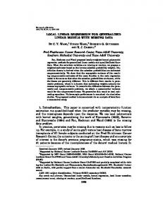
Estimated regression functions

Estimated regression functions

t')

+++ true regression function

+++ true regression function

r C\I

C\I

,

CD

'~~

f/)

c:

0 0f/)

l!!

:j

:~

CD

f/)

c:

0 0f/)

l!! 0

I i

i

i

-2

-1

0

1

2

x

+++ true regression function

CD

0

c: 0

0f/)

~

0

C\I

0 q 0

o Figure 5

0

l!!

-1

x

:1 CD

-2

Figure 4

Estimated regression functions

f/)

....

I

I

I

I

I

-2

-1

0

1

2

x Figure 6

2