Variable Impedance Control A Reinforcement Learning ... - CiteSeerX

Variable Impedance Control A Reinforcement Learning Approach Jonas Buchli, Evangelos Theodorou, Freek Stulp, Stefan Schaal

Abstract— One of the hallmarks of the performance, versatility, and robustness of biological motor control is the ability to adapt the impedance of the overall biomechanical system to different task requirements and stochastic disturbances. A transfer of this principle to robotics is desirable, for instance to enable robots to work robustly and safely in everyday human environments. It is, however, not trivial to derive variable impedance controllers for practical high DOF robotic tasks. In this contribution, we accomplish such gain scheduling with a reinforcement learning approach algorithm, PI2 (Policy Improvement with Path Integrals). PI2 is a model-free, sampling based learning method derived from first principles of optimal control. The PI2 algorithm requires no tuning of algorithmic parameters besides the exploration noise. The designer can thus fully focus on cost function design to specify the task. From the viewpoint of robotics, a particular useful property of PI2 is that it can scale to problems of many DOFs, so that RL on real robotic systems becomes feasible. We sketch the PI2 algorithm and its theoretical properties, and how it is applied to gain scheduling. We evaluate our approach by presenting results on two different simulated robotic systems, a 3-DOF Phantom Premium Robot and a 6-DOF Kuka Lightweight Robot. We investigate tasks where the optimal strategy requires both tuning of the impedance of the end-effector, and tuning of a reference trajectory. The results show that we can use path integral based RL not only for planning but also to derive variable gain feedback controllers in realistic scenarios. Thus, the power of variable impedance control is made available to a wide variety of robotic systems and practical applications.

I. I NTRODUCTION Biological motor systems excel in terms of versatility, performance, and robustness in environments that are highly dynamic, often unpredictable, and partially stochastic. In contrast to classical robotics, mostly characterized by high gain negative error feedback control, biological systems derive some of their superiority from low gain compliant control with variable and task dependent impedance. If we adapt this concept of adaptive impedance for PD negative feedback control, this translates into time varying proportional and derivative gains, also known as gain scheduling. Finding the appropriate gain schedule for a given task is, however, a hard problem. One possibility to overcome such problems is Reinforcement Learning (RL). The idea of RL is that, given only a reward function, the learning algorithm finds strategies that yield high reward through trial and error. As a special and important feature, RL accomplishes such optimal performance without knowledge of the models of the motor system and/or the environment. However, so far, RL does not scale well to high-dimensional continuous state-action control problems. Closely related to RL is optimal control theory, where gain scheduling is a natural part of many optimal control PREPRINT May 28, 2010 To appear in Proceedings RSS 2010 (c) 2010

algorithms. However, optimal control requires model-based derivations, such that it is frequently not applicable to complex robotic systems and environments, where models are unknown. In this paper, we present a novel RL algorithm that does scale to complex robotic systems, and that accomplishes gain scheduling in combination with optimizing other performance criteria. Evaluations on two simulated robotic systems demonstrate the effectiveness of our approach. In the following section, we will first motivate variable impedance control. Then, we sketch our novel RL algorithms, called PI2 , and its applicability to learning gain scheduling. In the fourth section, we will present evaluation results on a 3 DOF and a 6 DOF robotic arm, where the task requires the robot to learn both a reference trajectory and the appropriate time varying impedance. We conclude with a review of related work and discussions of future directions. II. VARIABLE

IMPEDANCE CONTROL

The classical approach to robot control is negative feedback control with high proportional-derivative (PD) gains. This type of control is straightforward to implement, robust towards modeling uncertainties, and computationally cheap. Unfortunately, high gain control is not ideal for many tasks involving interaction with the environment, e.g. force control tasks or locomotion. In contrast, impedance control [5] seeks to realize a specific impedance of the robot, either in end-effector or joint space. The issue of specifying the target impedance, however, is not completely addressed as of yet. While for simple factory tasks, where the properties of the task and environment are know a priori, suitable impedance characteristics may be derivable, it is usually not easy to understand how impedance control is applied to more complex tasks such as a walking robot over difficult terrain or the manipulation of objects in daily life (e.g. pillows, hammers, cans, etc.). An additional benefit of variable impedance behavior in a robot comes from the added active safety due to soft “giving in”, both for the robot and its environment. In the following we consider robots with torque controlled joints. The motor commands u are calculated via a PD control law with feedforward control term uf f : u = −KP (q − qd ) − KD (q˙ − q˙ d ) + uf f

(1)

where KP , KD are the positive definite position and velocity gain matrices, q, q˙ are the joint positions and velocities, and qd , q˙ d are the desired joint positions and velocities. The feedforward control term may come, for instance, from an

inverse dynamics control component, or a computed torque control component [15]. Thus, the impedance of a joint is parameterized by the choice of the gains KP (“stiffness”) and KD (“damping”). For many applications, the joint space impedance is, however, of secondary interest. Most often, regulating impedance matters the most at certain points that contact with the environment, e.g., the end-effectors of the robot. We therefore need to assess the impedance at these points of contacts rather than the joints. Joint space impedance is computed from the desired task space impedance KP,x , KD,x by help of the Jacobian J of the forward kinematics of the robot as follows [15]: KP,q = JT KP,x J and KD,q = JT KD,x J

(2)

Here we assume that the geometric stiffness due to the change of the Jacobian is negligible in comparison to the terms in Eq.(2). Regulating the task space impedance thus implies regulating the joint space impedance. Furthermore, this fundamental mathematical relationship between joint and task space also implies that a constant task stiffness in general means varying gains at the joint level. In the next section we will sketch a reinforcement learning algorithm that is applied to learning the time dependent gain matrices. III. R EINFORCEMENT THE

LEARNING IN HIGH DIMENSIONS

PI

2

–

ALGORITHM

Reinforcement learning algorithms can be derived from different frameworks, e.g., dynamic programming, optimal control, policy gradients, or probabilistic approaches. Recently, an interesting connection between stochastic optimal control and Monte Carlo evaluations of path integrals was made [9]. In [18] this approach is generalized, and used in the context of model-free reinforcement learning with parameterized policies, which resulted in the PI2 algorithm. In the following, we provide a short outline of the prerequisites and the development of the PI2 algorithm as needed in this paper. For more details refer to [18]. The foundation of PI2 comes from (model-based) stochastic optimal control for continuous time and continuous stateaction systems. We assume that the dynamics of the control system is of the form x˙ t = f (xt , t) + G(xt ) (ut + ǫt ) = ft + Gt (ut + ǫt )

(3)

with xt ∈ ℜn×1 denoting the state of the system, Gt = G(xt ) ∈ ℜn×p the control matrix, ft = f (xt ) ∈ ℜn×1 the passive dynamics, ut ∈ ℜp×1 the control vector and ǫt ∈ ℜp×1 Gaussian noise with variance Σǫ . Many robotic systems fall into this class of control systems. For the finite horizon problem ti : tN , we want to find control inputs uti :tN which minimize the value function V (xti ) = Vti = min Eτ i [R(τ i )] u ti :tN

PREPRINT May 28, 2010 To appear in Proceedings RSS 2010 (c) 2010

(4)

where R is the finite horizon cost over a trajectory starting at time ti in state xti and ending at time tN R(τ i ) = φtN +

Z

tN

rt dt

(5)

ti

and where φtN = φ(xtN ) is a terminal reward at time tN . rt denotes the immediate reward at time t. τ i are trajectory pieces starting at xti and ending at time tN . As immediate reward we consider 1 rt = r(xt , ut , t) = qt + uTt Rut 2

(6)

where qt = q(xt , t) is an arbitrary state-dependent reward function, and R is the positive semi-definite weight matrix of the quadratic control cost. From stochastic optimal control [16], it is known that the associated Hamilton Jacobi Bellman (HJB) equation is 1 ∂t Vt = qt + (∇x Vt )T ft − (∇x Vt )T Gt R−1 GTt (∇x Vt ) (7) 2
1 + trace (∇xx Vt )Gt Σǫ GTt 2 The corresponding optimal control is a function of the state and it is given by the equation: u(xti ) = uti = −R−1 GTti (∇xti Vti )

(8)

We are leaving the standard development of this optimal control problem by transforming the HJB equations with the substitution Vt = −λ log Ψt and by introducing a simplification λR−1 = Σǫ . In this way, the transformed HJB equation becomes a linear 2nd order partial differential equation. Due to the Feynman-Kac theorem [13, 25], the solution for the exponentially transformed value function becomes    Z N −1 X 1 qtj dtdτ i Ψti = lim p (τ i |xi ) exp − φtN + dt→0 λ j=0

(9) Thus, we have transformed our stochastic optimal control problem into an approximation problem of a path integral. As detailed in [18], it is not necessary to compute the value function explicitly, but rather it is possible to derive the optimal controls directly: Z P (τ i ) u (τ i ) dτ i (10) uti =
−1 (Gti ǫti − bti ) u(τ i ) = R−1 Gti T Gti R−1 Gti T

where P (τ i ) is the probability of a trajectory τ i , and bti is a more complex expression, beyond the space constraints of this paper. The important conclusion is that it is possible to evaluate Eq. (10) from Monte Carlo roll-outs of the control system, i.e., our optimal control problem can be solved as an estimation problem.

A. The PI2 Algorithm The PI2 algorithm is just a special case of the optimal control solution in Eq. (10), applied to control systems with parameterized control policy: at = gtT (θ + ǫt )

(11)

i.e., the control command is generated from the inner product of a parameter vector θ with a vector of basis function gt – the noise ǫt is interpreted as user controlled exploration noise. A particular case of a control system with parameterized policy is the Dynamic Movement Primitives (DMP) approach introduced by [6]: 1 v˙ t τ

1 q˙d,t τ ft 1 s˙ t τ [gt ]j wj

= ft + gtT (θ + ǫt )

TABLE I P SEUDOCODE OF THE PI2

•

•

(12)

Given: – An immediate cost function rt = qt + θT t Rθt (cf. Eq. (5)) – A terminal cost term φtN (cf. 5) – A stochastic parameterized policy at = gtT (θ + ǫt ) (cf. Eqs. (11) and (12)) – The basis function gti from the system dynamics (cf. 14) – The variance Σǫ of the mean-zero noise ǫt – The initial parameter vector θ Repeat until convergence of the trajectory cost R: – Create K roll-outs of the system from the same start state x0 using stochastic parameters θ + ǫt at every time step – For all K roll-outs, compute:
− 1 S(τ i,k ) ∗ P τ i,k = PKe λ − 1 S(τ ) i,k ] [e λ k=1

PN−1

qtj ,k + ∗ S(τ i,k ) = φtN ,k + j=i Mtj ,k ǫtj ,k )T R(θ + Mtj ,k ǫtj ,k )

= α(β(g − qd,t ) − vt )

∗ Mtj ,k =

(13)

R−1 gt ,k gtT ,k j j gT R−1 gt ,k tj ,k

1 2

PN−1

j=i+1

(θ +

j

– For all i time steps, compute:

(14)


 PK  P τ i,k Mti ,k ǫti ,k k=1 PN −1 (N−i) wj,ti [δ θti ]j i=0 PN −1 Compute [δθ]j =

∗ δθti =

(15)

The intuition of this approach is to create desired trajectories qd,t , q˙d,t , q¨d,t = τ v˙ t for a motor task out of the time evolution of a nonlinear attractor system, where the goal g is a point attractor and q0 the start state. The parameters θ determine the shape of the attractor landscape, which allows to represent almost arbitrary smooth trajectories, e.g., a tennis swing, a reaching movement, or a complex dance movement. While leaving the details of the DMP approach to [6], for this paper the important ingredients of DMPs are that i) the attractor system Eq. (12) has the same form as Eq. (3), and that ii) the p-dimensional parameter vector can be interpreted as motor commands as used in the path integral approach to optimal control. Learning the optimal values for θ will thus create a optimal reference trajectory for a given motor task. The PI2 learning algorithm applied to this scenario is summarized in Table I. As illustrated in [18, 19], PI2 outperforms previous RL algorithms for parameterized policy learning by at least one order of magnitude in learning speed and also lower final cost performance. As an additional benefit, PI2 has no open algorithmic parameters, except for the magnitude of the exploration noise ǫt (the parameter λ is set automatically, cf. [18]). We would like to emphasize one more time that PI2 does not require knowledge of the model of the control system or the environment. Key Innovations in PI2 : In summary we list the key innovations in PI2 that we believe lead to its superior performance. These innovations make applications like the the learning of gain schedules for high dimensional tasks possible. 2 • The basis of the derivation of the PI algorithm is the transformation of the optimal control problem from a constrained minimization to a maximum likelihood formulation. This transformation is very critical since there PREPRINT May 28, 2010 To appear in Proceedings RSS 2010 (c) 2010

1D PARAMETERIZED

P OLICY.

= vt

= −αst wj st (g − q0 ) = Pp k=1 wk
= exp −0.5hj (st − cj )2

ALGORITHM FOR A

–

i=0

wj,ti (N−i)

– Update θ ← θ + δθ – Create one noiseless roll-out to check the trajectory cost R = PN−1 rti . In case the noise cannot be turned off, i.e., a φt N + i=0 stochastic system, multiple roll-outs need to be averaged.

•

•

•

•

is no need to calculate a gradient that is usually sensitive to noise and large derivatives in the value function. Paths with higher cost have lower probability. A clear intuition that has also rigorous mathematical representation through the exponentiation of the value function. This transformation is necessary for the linearization of HJB into the Chapman-Kolmogorov PDE. With PI2 the optimal control problem is solved with the forward propagation of dynamics. Thus no backward propagation of approximations of the value function is required. This is a very important characteristic of PI2 that allows for sampling (i.e. roll-out) based estimation of the path-integral. For high dimensional problems, it is not possible to sample the whole state space and that is the reason for applying path integral control in an iterative fashion to update the parameters of the DMPs. The derivation of an RL algorithm from first principles largely eliminates the need for open parameters in the final algorithm. IV. VARIABLE I MPEDANCE C ONTROL

WITH

PI2

The PI2 algorithm as introduced above seems to be solely suited for optimizing a trajectory plan, and not directly the controller. Here we will demonstrate that this is not the case, and how PI2 can be used to optimize a gain schedule

simultaneously to optimizing the reference trajectory. For this purpose, it is important to realize how Eq. (3) relates to a complete robotics system. We assume a d DOF robot that obeys rigid body dynamics. qv denotes the joint velocities, and qp the joint angle positions. Every DOF has its own reference trajectory from a DMP, which means that Eqs. (12) are duplicated for every DOF, while Eqs. (13), (14), and (15) are shared across all DOFs – see [6] for explanations on how to create multi-dimensional DMPs. Thus, Eq. (3) applied to this context, i.e. using rigid body dynamics equations, with M, C, G the Inertia matrix, Coriolis/centripedal and and gravity forces respectively, becomes: q˙ v q˙ p 1 s˙ t τ where each ui

=

M(qp )−1 (−C(qp , qv ) − G(qp ) + u)

=

qv

=

−αst

element ui of the control vector u:   p
p v − ξi KP,i qiv − qd,i = −KP,i qip − qd,i

+

uf f,i

(16)

(17)

p v The terms qd,i , qd,i are the reference joint angle position and velocity of the ith DOF and they are given by the set of equations:

1 v p v q˙ = α(β(gi − qd,i ) − qd,i + gti,T (θiref + ǫit ) τ d,i 1 p v q˙ = qd,i (18) τ d,i Note that in the control law in (17), we used Eq. (1) applied to every DOF individually using a time varying gain, and i we inserted the common practice that the damping gain KD is written as the square root of the proportional gain KPi with a user determined multiplier ξ i . A critically important result of [18] is that for the application of PI2 only those differential equations in Eq. (16) matter that have learnable parameter θi . Moreover, the optimization of these parameters is accomplished by optimizing the parameter vector of each differential equation independently (as shown in Table I), despite that the DOFs are coupled through the cost function. For this reason, PI2 operates in a model free mode, as only one of the DMP differential equation per DOF is required, and all other equations, including the rigid body dynamics model, drop out. For variable stiffness control, we exploit these insights and add one more differential equation per DOF in Eq. (16):   i,T K˙ P,i = αK gt,K (θ iK + ǫiK,t ) − KP,i (19) wj (20) [gt,K ]j = Pp k=1 wk This equation models the time course of the position gains, coupled to Eq. (15) of the DMP. Thus, KP,i is represented by a basis function representation linear with respect to the learning parameter θiK , and these parameter are learned with the PI2 algorithm following Table I. We will assume that the PREPRINT May 28, 2010 To appear in Proceedings RSS 2010 (c) 2010

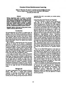
Fig. 1.

3-DOF Phantom simulation in SL.

time constant α1K is so small, that for all practical purposes we i,T can assume that KP,i = gt,K (θ iK + ǫiK,t ) holds at all times. Essentially equations 16,17,18 and 20 are incorporated in one stochastic dynamical system of the form of Eq. (3). In conclusion, we achieved a novel formulation of learning both the reference trajectory and the gain schedule for a multidimensional robotic system with model-free reinforcement learning, using the PI2 algorithm and its theoretical properties as foundation of our derivations. V. R ESULTS We will now present results of applying the outlined algorithms to two simulated robot arms with 3 and 6 DOFs, respectively. For both robots, the immediate reward at time step t is given as: rt = Wgain

X

i KP,t + Wacc ||¨ x|| + Wsubgoal C(t)

(21)

i

P i is the sum over the proportional gains over Here, i KP,t all joints. The reasoning behind penalizing the gains is that low gains lead to several desirable properties of the system such as compliant behavior (safety and/or robustness [2]), lowered energy consumption, and less wear and tear. The term ||¨ x|| is the magnitude of the accelerations of the end-effector. This quantity is penalized to avoid high-jerk end-effector motion. This penalty is low in comparison to the gain penalty. The robot’s primary task is to pass through an intermediate goal, either in joint space or end-effector space – such scenarios occur in tasks like playing tennis or table tennis. The component of the cost function C(t) that represents this primary task will be described individually for each robot in the next sections. Gains and accelerations are penalized at each time step, but C(t) only leads to a cost at specific time steps along the trajectory. For both robots, the cost weights are Wsubgoal = 2000, Wgain = 1/N , Wacc = 1/N . Dividing the weights by the number of time steps N is convenient, as it makes the weights independent of the duration of a movement. A. Robot 1: 3-DOF Phantom The Phantom Premium 1.5 Robot is a 3 DOF, two link arm. It has two rotational degrees of freedom at the base and one in

Fig. 2. Initial (red, dashed) and final (blue, solid) joint trajectories and gain scheduling for each of the three joints of the phantom robot. Yellow circles indicate intermediate subgoals.

the arm. We use a physically realistic simulation of this robot generated in SL [14], as depicted in Fig. 1. The task for this robot is intentionally simple and aimed at demonstrating the ability to tune task relevant gains in joint space with straightforward and easy to interpret data. The duration of the movement is 2.0s, which corresponds to 1000 time steps at 500Hz servo rate. The intermediate goals for this robot are set as follows: C(t) = δ(t − 0.4) · δ(t − 0.8) · δ(t − 1.2) ·

| qSR (t) + 0.2 | + | qSF E (t) − 0.4 | +

(22)

This penalizes joint SR for not having an angle qSR = −0.2 at time t = 0.4s. Joints SFE and EB are also required to go through (different) intermediate angles at times 0.8s and 1.2s respectively. The initial parameters θi for the reference trajectory are determined by training the DMPs with a minimum jerk trajectory [26] in joint space from qt=0.0 = [0.0 0.3 2.0]T to qt=2.0 = [−0.6 0.8 1.4]T . The function approximator for the proportional gains of the 3 joints is initialized to return a constant gain of 6.0N m/rad. The initial trajectories are depicted as red, dashed plots in Fig. 2, where the angles and gains of the three joints are plotted against time. Since the task of PI2 is to optimize both trajectories and gains with respect to the cost function, this leads to a 6-D RL problem. The robot executes 100 parameter updates, with 4 noisy exploration trials per update. After each update, we perform one noise-less test trial for evaluation purposes. Fig. 3 depicts the learning curve for the phantom robot (left), which is the overall cost of the noise-less test trial after each parameter update. The joint space trajectory and gain scheduling after 100 updates are depicted as blue, solid lines in Fig. 2. PREPRINT May 28, 2010 To appear in Proceedings RSS 2010 (c) 2010

Fig. 3.

Learning curve for the phantom robot.

| qEB (t) − 1.5 | From these graphs, we draw the following conclusions: •

•

•

PI2 has adapted the initial minimum jerk trajectories such that they fulfill the task and pass through the desired joint angles at the specified times with only small error. These intermediate goals are represented by the circles on the graphs. The remaining error is a result of the trade-off between the different factors of the cost function (i.e. penalty for distance to goal vs. penalty for high gains). Because the magnitude of gains is penalized in general, they are low when the task allows it. After t = 1.6s, all gains drop to the minimum value1 , because accurate tracking is no longer required to fulfill the goal. Once the task is completed, the robot becomes maximally compliant, as one would wish it to be. When the robot is required to pass through the intermediate targets, it needs better tracking, and therefore higher gains. Therefore, the peaks of the gains correspond

1 We bound the gains between pre-specified maximum and minimum values. Too high gains would generate oscillations and can lead to instabilities of the robot, and too low gains lead to poor tracking such that the robot frequently runs into the joint limits.

Fig. 4.

Initial (red, dotted), intermediate (green, dashed), and final (blue, solid) end-effector trajectories of the Kuka robot.

roughly to the times where the joint is required to pass through an intermediate point. • Due to nonlinear effects, e.g., Coriolis and centripedal forces, the gain schedule shows more complex temporal behavior as one would initially assume from specifying three different joint space targets at three different times. In summary, we achieved the objective of variable impedance control: the robot is compliant when possible, but has a higher impedance when the task demands it. B. Robot 2: 6-DOF Kuka robot Next we show a similar task on a 6 DOF arm, a Kuka LightWeight Arm. This example illustrates that our approach scales well to higher-dimensional systems, and also that appropriate gains schedules are learned when intermediate targets are chosen in end-effector space instead of joint space. The duration of the movement is 1.0s, which corresponds to 500 time steps. This time, the intermediate goal is for the end-effector x to pass through [ 0.7 0.3 0.1]T at time t = 0.5s: C(t) =

δ(t − 0.5)| x − [ 0.7 0.3 0.1]T |

•

(23)

The six joint trajectories are again initialized as minimum jerk trajectories. As before, the resulting initial trajectory is plotted as red, dashed line in Fig. 4. The initial gains are set to a constant [60, 60, 60, 60, 25, 6]T . Given these initial conditions, finding the parameter vectors for DMPs and gains that minimizes the cost function leads to a 12-D RL problem. We again perform 100 parameter updates, with 4 exploration trials per update. The learning curve for this problem is depicted in Fig. 5. The trajectory of the end-effector after 30 and 100 updates is depicted in Fig. 4. The intermediate goal at t = 0.5 is visualized by circles. Finally, Fig. 6 shows the gain schedules after 30 and 100 updates for the 6 joints of the Kuka robot. From these graphs, we draw the following conclusions: 2 • PI has adapted joint trajectories such that the endeffector passes through the intermediate subgoal at the right time. It learns to do so after only 30 updates (Figure 5). • After 100 updates the peaks of most gains occur just before the end-effector passes through the intermediate goal (Figure 6), and in many cases decrease to the PREPRINT May 28, 2010 To appear in Proceedings RSS 2010 (c) 2010

Fig. 5.

•

Learning curve for the Kuka robot.

minimum gain directly afterwards. As with the phantom robot we observe high impedance when the task requires accuracy, and more compliance when the task is relatively unconstrained. The second joint (GA2) has the most work to perform, as it must support the weight of all the more distal links. Its gains are by far the highest, especially at the intermediate goal, as any error in this DOF will lead to a large endeffector error. The learning has two phases. In the first phase (plotted as dashed, green), the robot is learning to make the end-effector pass through the intermediate goal. At this point, the basic shape of the gain scheduling has been determined. In the second phase, PI2 fine tunes the gains, and lowers them as much as the task permits. VI. R ELATED WORK

In optimal control and model based RL, Differential Dynamic Programming (DDP) [7] has been one of the most established and used frameworks for finite horizon optimal control problems. In DDP, both state space dynamics and cost function are approximated up to the second order. The assumption of stabilizability and detectability for the local approximation of the dynamics are necessary for the convergence of DDP. The resulting state space trajectory is locally optimal while the corresponding control policy consists of open loop feedforward command and closed loop gains relative to a nominal and optimal final trajectory. This characteristic allows the use of DDP for both planning and control gain scheduling problems.

Fig. 6. Initial (red, dotted), intermediate (green, dashed), and final (blue, solid) joint gain schedules for each of the six joints of the Kuka robot.

In [4, 24] DDP was extended to incorporate constrains in state and controls. In [10] the authors suggest computational improvements to constrained DDP and apply the proposed algorithm to a low dimensional planning problem. An example of a DDP application to robotics is in [12]. In this work, a min-max or Differential Game Theory approach to optimal control is proposed. There is a strong link between robust control frequency design analysis such as H∞ control and the framework of Differential Game Theory [1]. Essentially the min-max DDP results in robust feedback control policies with respect to model uncertainty and unknown dynamics. Although, in theory, min-max DDP should resolve the issue of model uncertainty, it can lead to overly conservative control policies. The conservatism results from the need to guarantee that the game theoretic approach will be always stabilizable, i.e. making sure that the stabilizing controller wins. For linear PREPRINT May 28, 2010 To appear in Proceedings RSS 2010 (c) 2010

and time invariant systems, such guarantee is feasible through γ-iteration [23]. However, for nonlinear systems providing this guarantee is not trivial. The work on Receding Horizon DDP [17] provided an alternative and rather efficient way of computing local optimal feedback controls. Nevertheless, all the computations of optimal trajectories and control take place off-line and the model predictive component is only due to the fact that the final target state of the optimal control problem varies. Recent work on LQR-trees uses a simpler variation of DDP, the iterative Linear Quadratic Regulator (iLQR) [11], which is based on linear approximations of the state space dynamics, in combination with tools from Nonlinear Robust Control theory for region of attraction analysis. Given the local optimal feedback control policies, the sums of squares optimization scheme is used to quantify the size of of the basin of attraction, and provides so-called control funnels. These funnels improve sampling since they quantize the state space into attractor regions placed along the trajectories towards the target state. This is a model based approach and inherits all the problems of model based approaches to optimal control. In addition, even though sampling is improved, it is still an issue how LQR trees scale in high dimensional dynamical systems. The path integral formalism for optimal control was introduced in [8, 9]. In this work, the role of noise in symmetry breaking phenomena was investigated in the context of stochastic optimal control. In [22] the path integral formalism is extended for stochastic optimal control of multi-agent systems, which is not unlike our multi degree-of-freedom control systems. Recent work on stochastic optimal control by [21, 20, 3] shows that for a class of discrete stochastic optimal control problems, the Bellman equation can be written as the KL divergence between the probability distribution of the controlled and uncontrolled dynamics. Furthermore, it is shown that the class of discrete KL divergence control problem is equivalent to the continuous stochastic optimal control formalism with quadratic cost control function and under the presence of Gaussian noise. In all this aforementioned work, both in the path integral formalism as well as in KL divergence control, the class of stochastic dynamical systems under consideration is rather restrictive since the control transition matrix is state independent. Moreover, the connection to direct policy learning in RL and model-free learning was not made in any of the previous projects. In [3], the stochastic optimal control problem is investigated for discrete state-action spaces, and therefore it is treated as Markov Decision Process (MDP). To apply our PI2 algorithm, we do not discretize the state space and we do not treat the problem as an MDP. Instead we work in continuous state-action spaces which are suitable for performing RL in high dimensional robotic systems. To the best of our knowledge, our results present RL in one of the most high dimensional continuous state action spaces. In our derivations, the probabilistic interpretation of control comes directly from the Feynman-Kac Lemma. Thus we do not have to impose any artificial pseudo-probability treatment

of the cost as in [3]. In addition, for continuous state-action spaces, we do not have to learn the value function as it is suggested in [3] via Z-learning. Instead we directly obtain the controls based on our generalization of optimal controls. In the previous work, the problem of how to sample trajectories is not addressed. Sampling is performed with the hope to cover all the relevant state space. We follow a rather different approach by incremental updating that allows to attack robotic learning problems of the complexity and dimensionality of complete humanoid robots. VII. D ISCUSSION We presented a model-free reinforcement learning approach that can learn variable impedance control for robotic systems. Our approach is derived from stochastic optimal control with path integrals, a relatively new development that transforms optimal control problems into estimation problems. In particular, our PI2 algorithm goes beyond the original ideas of optimal control with path integrals by realizing the applicability to optimal control with parameterized policies and model-free scenarios. The mathematical structure of the PI2 algorithm makes it suitable to optimize simultaneously both reference trajectories and gain schedules. This is similar to classical differential dynamic (DDP) programming methods, but completely removes the requirements of DDP that the model of the controlled system must be known, that the cost function has to be twice differentiable in both state and command cost, and that the dynamics of the control system have to be twice differentiable. The latter constraints make it hard to apply DDP to movement tasks with discrete events, e.g., as typical in force control and locomotion. We evaluated our approach on two simulated robot systems, which posed up to a 12 dimensional learning problems in continuous state-action spaces. The goal was to learn compliant control while fulfilling kinematic task constraints, like passing through an intermediate target. The evaluations demonstrated that the algorithm behaves as expected: it increases gains when needed, but tries to maintain low gain control otherwise. The optimal reference trajectory always fulfilled the task goal. Learning speed was rather fast, i.e., within at most a few hundred trials, the task objective was accomplished. From a machine learning point of view, this performance of a reinforcement learning algorithm is very fast. The PI2 algorithms inherits the properties of all trajectorybased learning algorithms in that it only finds locally optimal solutions. For high dimensional robotic system, this is unfortunately all one can hope for, as exploring the entire state-action space in search for a globally optimal solution is impossible. Future work will apply the suggested methods on actual robots for mobile manipulation and locomotion controllers. We believe that our methods are a major step towards realizing compliant autonomous robots that operate robustly in dynamic and stochastic environment without harming other beings or themselves. PREPRINT May 28, 2010 To appear in Proceedings RSS 2010 (c) 2010

R EFERENCES [1] T. Basar and P. Bernhard. H-Infinity Optimal Control and Related Minimax Design Problems: A Dynamic Game Approach. Birkh¨auser, Boston, 1995. [2] J. Buchli, M. Kalakrishnan, M. Mistry, P. Pastor, and S. Schaal. Compliant quadruped locomotion over rough terrain. In IEEE/RSJ International Conference on Intelligent Robots and Systems, pages 814–820, 2009. [3] Todorov E. Efficient computation of optimal actions. Proc Natl Acad Sci USA, 106(28):11478–83, 2009. [4] R. Fletcher. Practical Methods of Optimization, volume 2. Wiley, 1981. [5] N. Hogan. Impedance control - an approach to manipulation. I - theory. II - implementation. III - applications. ASME, Transactions, Journal of Dynamic Systems, Measurement, and Control, 107:1–24, 1985. [6] A.J. Ijspeert. Vertebrate locomotion. In M.A. Arbib, editor, The handbook of brain theory and neural networks, pages 649–654. MIT Press, 2003. [7] D. H. Jacobson and D. Q. Mayne. Differential Dynamic Programming. Optimal Control. Elsevier Publishing Company, New York, 1970. [8] H. J. Kappen. Linear theory for control of nonlinear stochastic systems. Phys Rev Lett, 95(20):200201, 2005. [9] H.J. Kappen. Path integrals and symmetry breaking for optimal control theory. Journal of Statistical Mechanics: Theory and Experiment, 2005(11):P11011, 2005. [10] G. Lantoine and R.P. Russell. A hybrid differential dynamic programming algorithm for robust low-thrust optimization. In AAS/AIAA Astrodynamics Specialist Conference and Exhibit, 2008. [11] W. Li and E. Todorov. Iterative linear quadratic regulator design for nonlinear biological movement systems. In Proceedings of the 1st International Conference on Informatics in Control, Automation and Robotics, pages 222–229, 2004. [12] J. Morimoto and C. Atkeson. Minimax differential dynamic programming: An application to robust biped walking. In In Advances in Neural Information Processing Systems 15, pages 1563–1570. MIT Press, Cambridge, MA, 2002. [13] B. K. Oksendal. Stochastic differential equations: an introduction with applications. Springer, Berlin, New York, 6th edition, 2003. [14] S. Schaal. The SL simulation and real-time control software package. Technical report, University of Southern California, 2007. [15] L. Sciavicco and B. Siciliano. Modelling and Control of Robot Manipulators. Springer, London, New York, 2000. [16] R.F. Stengel. Optimal Control and Estimation. Dover Publications, New York, 1994. [17] Y. Tassa, T. Erez, and W. Smart. Receding horizon differential dynamic programming. In Advances in Neural Information Processing Systems 20, pages 1465–1472. MIT Press, Cambridge, MA, 2008. [18] E. Theodorou, J. Buchli, and S. Schaal. Reinforcement learning in high dimensional state spaces: A path integral approach. Journal of Machine Learning Research, 2010. Accepted for publication. [19] E. Theodorou, J. Buchli, and S. Schaal. Reinforcement learning of motor skills in high dimensions: A path integral approach. In Proceedings of the IEEE International Conference on Robotics and Automation, 2010. [20] E. Todorov. Linearly-solvable markov decision problems. In Advances in Neural Information Processing Systems 19, pages 1369–1376. MIT Press, Cambridge, MA, 2007. [21] E. Todorov. General duality between optimal control and estimation. In Proceedings of the 47th IEEE Conference on Decision and Control, 2008. [22] B. van den Broek, W. Wiegerinck, and B. Kappen. Graphical model inference in optimal control of stochastic multi-agent systems. Journal of Artificial Intelligence Research, 32:95–122, 2008. [23] T. Vincent and W. Grantham. Non Linear And Optimal Control Systems. John Wiley & Sons Inc., 1997. [24] S. Yakowitz. The stagewise Kuhn-Tucker condition and differential dynamic programming. IEEE Transactions on Automatic Control, 31(1):25–30, 1986. [25] J. Yong. Relations among ODEs, PDEs, FSDEs, BSDEs, and FBSDEs. In Proceedings of the 36th IEEE Conference on Decision and Control, 1997, volume 3, pages 2779–2784, Dec 1997. [26] M. Zefran, V. Kumar, and C.B. Croke. On the generation of smooth three-dimensional rigid body motions. IEEE Transactions on Robotics and Automation, 14(4):576–589, 1998.