Color profile: Disabled Composite Default screen
71
Variance and efficiency of the combined estimator in incomplete block designs of use in forest genetics: a numerical study Beatriz Villanueva and Javier Moro
Abstract: The efficiency of combined interblock–intrablock and intrablock analysis for the estimation of treatment contrasts in alpha designs is compared using Monte-Carlo simulation. The combined estimator considers treatments and replications as fixed effects and blocks as random effects, whereas the intrablock estimator considers treatments, replications, and blocks as fixed effects. The variances of the estimators are used as the criterion for comparison. The combined estimator yields more accurate estimates than the intrablock estimator when the ratio of the block to the error variance is small, especially for designs with the fewest degrees of freedom. The accuracy of both estimators is similar when the ratio of variances is large. The variance of the combined estimator is very close to that of the best linear unbiased estimator except for designs with small number of replicates and families or provenances. Approximations commonly used for the variance of the combined estimator when variances of the random effects are unknown are studied. The downward or negative bias in the estimates of the variance given by the standard approximation used in statistical packages is largest under the conditions in which the combined estimator is more efficient than the intrablock estimator. Estimates of the relative efficiency of combined estimators have an upward bias that can exceed 10% of the true value in small- and middle-sized designs with two or three replicates. In designs with four or more replicates, often used in forest genetics, the bias is negligible. Résumé : Nous avons comparé, à l’aide d’une simulation Monte Carlo, l’efficacité des analyses combinées inter-bloc – intra-bloc et intra-bloc dans l’estimation des contrastes de traitements dans des dispositifs alpha. L’estimateur combiné considère les traitements et les répétitions comme des effets fixés et les blocs comme des effets aléatoires, alors que l’estimateur intra-bloc considère les traitements, les répétitions, ainsi que les blocs comme des effets fixés. Les variances des estimateurs sont utilisées comme critère de comparaison. L’estimateur combiné produit des estimés plus précis que l’estimateur intra-bloc lorsque le ratio de variance des blocs par rapport à l’erreur est faible, particulièrement pour les dispositifs avec le plus faible nombre de degrés de liberté. La précision des deux estimateurs est similaire lorsque le ratio des variances est élevé. La variance de l’estimateur combiné est très rapprochée de celle du meilleur estimateur linéar non-biasé sauf pour les dispositifs avec peu de répétitions, de familles ou de provenances. Nous avons étudié les approximations couramment utilisées pour la variance de l’estimateur combiné, lorsque les variances des effets aléatoires sont inconnues. La sous-estimation des estimés de la variance obtenue avec l’approximation standard utilisée dans des progiciels de statistique est à son maximum lorsque l’estimateur combiné est plus efficace que l’estimateur intrabloc. Les estimés de l’efficacité relative des estimateurs combinés peuvent excéder de plus de 10% les vraies valeurs dans des dispositifs dont la dimension est de petite à moyenne avec deux ou trois répétitions. Dans les dispositifs avec quatre répétitions ou plus, souvent utilisés en génétique forestière, le biais est négligeable. [Traduit par la Rédaction]
Villanueva and Moro
Introduction Many field experiments are carried out each year for selection of the best plant material. Selection can be among genotypes, varieties, provenances, families, etc, and these will be called generically treatments. The most popular experimental design for selection purposes has been randomReceived April 17, 2000. Accepted September 15, 2000. Published on the NRC Research Press website on December 19, 2000. B. Villanueva. Scottish Agricultural College, West Mains Road, Edinburgh EH9 3JG, Scotland, U.K. J. Moro.1 Unit of Forest Genetics, CIFOR-INIA, Apdo 8111, 28080 Madrid, Spain. 1
Corresponding author. e-mail:
[email protected]
Can. J. For. Res. 31: 71–77 (2001)
I:\cjfr\cjfr31\cjfr-01\X00-138.vp Friday, December 15, 2000 10:59:59 AM
77
ized complete block (RCB). However, when the number of treatments is large, RCBs occupy too much field space, they are difficult to lay out, and they have the risk of being too heterogeneous. The effectiveness of blocking is thus reduced. Incomplete block designs (IB), such as square and rectangular lattices, offer the possibility of reducing the size of blocks with an increase of the precision of intrablock comparisons. In the past, the problem was that these lattices were not available for all values of the number of treatments. Alpha-lattice designs were introduced by Patterson and Williams (1976) in an attempt to reduce restrictions on the number of treatments. Alpha lattices are binary, equireplicate, and proper (equal block size) IB designs. They have the important practical and theoretical property of being resolvable, i.e., the incomplete blocks can be grouped into superblocks, which are complete replicates (John and Williams 1994). This kind of IB has become widely used in
DOI:10.1139/cjfr-31-1-71
© 2001 NRC Canada
Color profile: Disabled Composite Default screen
72
agronomic variety testing when the number of varieties is large (>15). Williams and Matheson (1994) recommend their use in forest genetics trials, which normally intend to compare a large number of treatments. In many trials, substantial gains have been found in the relative efficiency (RE) of IB over RCB for estimating a particular treatment contrast (RE defined as the variance of the estimate in RCB divided by the variance in IB). Recently, Fu et al. (1998) have reported an efficiency of 1.25 of IB relative to RCB in a large number of Douglas-fir (Pseudotsuga menziesii (Mirb.) Franco) progeny trials in British Columbia. The effect of continuous or patchy environmental variation and of missing observations produced by natural or genetic mortality on the usual estimates from alpha lattices has also been studied using simulation by Fu et al. (1999a, 1999b). However, as variances are unknown they have to be estimated in each case to obtain an estimated relative efficiency (ERE). As “usual variance estimates are naive, i.e., too small,” not taking into account all sources of variability, reported EREs may be optimistic (Magnussen 1993). Treatment contrasts from an alpha design, and in general from an incomplete block design, can be estimated from intrablock analysis or from combined interblock–intrablock analysis. Intrablock analysis considers blocks as a fixed factor. This may result in the loss of information about treatments contained in the block totals. Combined analysis considers blocks as a random factor and allows the recovery of this information between blocks (Yates 1940). Intrablock analysis has the advantage of simplicity, but the correct inter- and intra-block randomization justifies treating blocks as a random factor (e.g., Calinski and Kageyama 1996). If the variance–covariance matrix of random effects is known, the combined estimator is the best linear unbiased estimator (BLUE), i.e., it has the smallest variance within the class of all linear unbiased estimators. However, in practice, variance components are unknown and have to be estimated. If estimates of variance components are substituted for their true values, then combined estimators of estimable functions of fixed effects are still unbiased under mild conditions. However, they are no longer best and their variances, which depend on the variance component estimators, are in general mathematically intractable. The usual current procedure of analysis, such as provided by SAS® PROC MIXED, obtains residual maximum likelihood (REML) estimates of the variance components, substitutes them for the parameter values, and then uses generalized least squares to produce combined estimates of contrasts and their variance. This procedure, however, underestimates the exact variance of the estimator, because it assumes that the variance component estimates are fixed. To correct for this bias, Kackar and Harville (1984) proposed an approximation for the variance of the combined estimator. The performance of this approximation and its proposed estimates have been studied for alpha lattices by Villanueva and Moro (1992). The objectives of this study were to quantify, through Monte-Carlo simulation, the advantage of the combined interblock–intrablock estimator of treatment contrasts over the relatively simpler intrablock estimator and to evaluate the bias in variance estimates and in the relative efficiency of these estimators in alpha-lattice designs.
Can. J. For. Res. Vol. 31, 2001
Estimation of contrasts Combined interblock–intrablock estimator Let yijl represent the observation for the ith treatment in the lth block of the jth replicate. Consider the following mixed model to represent these observations: [1]
yijl = µ + τi + ρ j + bjl + eijl
where µ is the overall mean, τi is the fixed effect of the ith treatment (i = 1, 2, ÿ, v), ρij is the fixed effect of the jth replicate (j = 1, 2, ÿ, r), bjl is the random effect of the lth block within the jth replicate (l = 1, 2, ÿ, s), and eijl is the random residual effect. In matrix form, eq. 1 can be written as [2]
y = 1µ + X1τ + X2 ρ + Zb + e
where y is a column vector of all N observations; 1 is a column vector of ones of order N; X1, X2, and Z are the treatment, replication, and block design matrices, respectively; τ and are the vectors of treatment and replicate effects; b is the vector of block effects with E(b) = 0 and V(b) = I bσ 2b ; and e is a N × 1 vector of residual effects with E(e) = 0 and V(e) = I N σ 2e and uncorrelated with b. Let U represent the incidence matrix of the fixed effects . Then, the model can be rewritten as [3]
y = U
+ Zb + e
with E(y) = U and V(y) = V = Hσ 2e , where H = ZZ′γ + IN σ2 and γ = b2 is the ratio of variances. Therefore, V is a funcσe tion, V(), of the parameter vector = (γ, σ 2e )′. Assume we want to estimate a linear combination of the elements of , say Φ = c′ with c′ = t′U. A BLUE of Φ can $ () = c ′ ␣ $ , where ␣ $ is a solution to the be obtained from Φ c mixed model equations: [4]
U ′ U U ′ Z ␣ U ′ y = −1 Z′ U Z′ Z + I γ b Z′ y
Let some generalized inverse of the coefficient matrix in eq. 4 be [5]
C () C01() C() = 00 C10() C11()
Thus the variance of the estimator is (Harville 1976a) [6]
$ ()] = c ′ C () c σ 2 V = [Φ c 00 e
$ () and Knowledge of is therefore necessary to obtain Φ c its variance. In practice, only estimates of are available. An estimator of Φ is obtained by replacing an estimate of for $ ( $ its true value. The resulting estimator, Φ c ), is unbiased for $ all usual estimates (y) of variance components (Kackar and Harville 1984), but its variance can be affected. This variance is in general intractable and usually approximated by substituting $ for in eq. 6. Though consistent, this approxi$ ( $ mation, V$ [Φ c )], underestimates in average the exact vari-
© 2001 NRC Canada
I:\cjfr\cjfr31\cjfr-01\X00-138.vp Friday, December 15, 2000 11:00:00 AM
Color profile: Disabled Composite Default screen
Villanueva and Moro $ ( $ ance, V [Φ c )], because it does not take into account the extra variation due to estimating (e.g., see Christensen 1991, p. 285).
Intrablock estimator Intrablock analysis considers block as a fixed effect. The model in this case is [7]
y = W + e
where W = (U, Z) and  = (␣′, b′)′. The expectation vector and variance–covariance matrix of y are E(y) = W and V(y) = I N σ 2e . Let ΦI = c I′  and c I′ = (c ′, 0 ′ ) . The intra$ = c ′ (W′ W)W′ y and block estimator of this contrast is Φ I I the variance is [8]
$ ) = c ′ (W′ W) − c σ 2 V (Φ I I I e
Thus, no knowledge of is required to obtain the estimator. However, σ 2e must be known to compute its variance. If σ 2e is unknown, then an unbiased estimate, σ$ 2e , can be substituted for σ 2e in eq. 8 to provide an unbiased estimate of the variance under both mixed and fixed effects (intrablock) models. In practice, the intrablock estimator is reduced to the RCB estimator if blocks appear to be nonsignificant at some significance level, say 5%, and they are not included in the model. If one proceeds in this way, one obtains what could $ ( $ be called an intrablock modified estimator Φ im ) .
Monte-Carlo simulation The statistical model used in the simulations was eq. 1 with µ = 10, τi = 0, for all i = 1, 2, ÿ, v, and ρ j = 0, for all j = 1, 2, ÿ, r. Observations were generated from [9]
y = 10 + v1 σ b + v 2σ e
where v1 and v2 are independent standard normal deviates. Different values (0.1, 0.5, 1.0, 5.0, and 10.0) were given to σ 2b , whereas σ 2e was set to 1 in all cases, with no loss of generality. Several alpha designs were chosen with varying values of the number of treatments, v; of replicates, r; and of blocks within replicates, s. Designs were constructed following Patterson and Williams (1976). Some related nonproper designs were also considered. For the chosen nonproper designs, the difference in block sizes was no more than one plot. All designs had 0 or 1 for concurrence in the same block of any two treatments. Estimates of variance components were obtained from equating standard ANOVA mean squares to their expected values under the mixed model. The quadratic forms used were the residual sum of squares under the fixed effects model (SSE) and the residual sum of squares under the model resulting from omitting the block factor (SSERB). The latter corresponds to a randomized complete block design. Let MSE and MSERB be the mean squares corresponding to SSE and SSERB, respectively. Unbiased estimates of the components were obtained from [10]
σ$ 2e = MSE
73
and v −1
σ$ 2b = (MSE RB − MSE)
s
v−
1 ∑ kl2 v l =1
where kl is the number of plots in the lth block. An estimate σ$ 2 of γ was obtained from γ$ = b2 . σ$ e Initially, the method provides unbiased estimates of the variance components (e.g., Searle et al. 1992). However, a bias is introduced since negative estimates of σ 2b are truncated to zero. The model is then equivalent to that of a RCB. The estimator of γ is inherently biased because it is a ratio of random variables. Alternatively, other methods of estimating the variance components, as the popular REML, can be used. Three treatment contrasts are considered, due to their practical interest: [11]
Φ = τ1 − 1
∑ τi
i= 2
v −1
,
Φ 2 = τa − τb
and Φ 3 = τa ′ − τb ′ where the subscripts a and b represent two treatments whose difference has minimum variance and subscripts a′ and b′ represent two treatments whose difference has maximum variance. Estimates of the three contrasts were obtained from both intrablock and combined interblock–intrablock analysis of each run. As already mentioned, negative estimates of γ were truncated to zero and the combined analysis reduced to that of a randomized complete block (RCB) design. Com$ ( $ $ bined and intrablock estimators (Φ c ) and ΦI ) as well as $ ( $ $ $ V [Φc ()] the “true” variance of the former (variance of Φ c ), computed as the variance of the empirical frequency distribution produced by the simulation) were obtained. The “true” variance is our best available approximation to the exact variance (unknown variance of the theoretical infinite population). The number of simulation runs for each design was taken equal to 40 000 to cover the true variance within an interval of half-length equal to 1.4% of the estimate with confidence coefficient of 0.95, under the assumptions. The traditional (standard) estimate of the variance of the com$ ( $ bined estimator, V$ [Φ c )] , was obtained for each run. Then, $ ( $ it was approximated by V$ [Φ c )], the mean over all runs. The variances of the intrablock estimator and of the combined estimator assuming known were computed from eqs. 8 and 6.
Results Intrablock versus combined analysis Figure 1 illustrates the comparison among “true” variances of the intrablock (from eq. 8), the intrablock modified and the combined estimators of contrast Φ3 for different val© 2001 NRC Canada
I:\cjfr\cjfr31\cjfr-01\X00-138.vp Friday, December 15, 2000 11:00:00 AM
Color profile: Disabled Composite Default screen
74
Can. J. For. Res. Vol. 31, 2001
Fig. 1. Minimum variance (BLUE) and “true” variances of the combined, intrablock modified, and intrablock estimators of contrast Φ 3 for different values of γ and different designs (r). In all cases, v = 20 and s = 5. Points labeled with a circle correspond to the variance of the combined estimator using REML estimates of the variance components (only for r = 2). Remaining points were obtained using ANOVA estimates of the variance components.
ues of γ and designs with v = 20. As expected, the combined analysis was substantially more efficient (i.e., estimated with lower variance) than intrablock analysis except when γ is $ ( $ large (γ ≥ 5.0). In general, the relative superiority of Φ c ) decreases with a higher number of replicates and treatments. $ ( $ For γ = 0.1, Φ c ) resulted in average about 20% more efficient than the intrablock estimator. Its advantage ranged from less than 2 to almost 40%. For γ = 0.5 and γ = 1.0, the average advantage was about 12 and 8%, respectively. Both estimates were similar when γ is large. Thus, for γ = 10.0, $ ( $ the improvement provided by Φ c ) averaged less than 0.6% for all designs and parameters considered. The possible advantages of using REML estimates of the variance components are difficult to evaluate analytically as their distribution in small samples is unknown. We obtained, by simulation, empirical frequency distributions of ANOVA and of REML estimates of γ, and they were found to be very close. For instance, for v = 20, r = 2, γ = 0.5 the 10, 25, 50, 75, 90 percentiles of these distributions were 0.0, 0.117, 0.481, 1.058, 1.810, respectively, for ANOVA and 0.0, 0.111, 0.477, 1.060, 1.820, respectively, for REML. Moreover, the differences between the variances of the combined estimator using the REML and the ANOVA estimates were very small (see case r = 2 in Fig. 1). The minimum variance of an unbiased estimator (variance of BLUE; i.e., assuming is known) as well as the variance of the intrablock estimator, which does not vary with γ, are also plotted for comparison. For low values of γ, the vari$ ( $ ances of the Φ im ) estimator are reduced with respect the intrablock estimator, but they are always higher than that of $ ( $ the combined estimator. For medium values of γ, the Φ im ) estimator is even more inefficient than the intrablock estima-
tor. When γ is high, the differences among variances of estimators are small. Approximations to the exact variance of the combined estimator $ ( $ $ $ The “true” variance of Φ c ), V [Φc ()] is compared with the variance obtained by substituting $ for in eq. 6. A measure $ ( $ of the bias in estimating V [Φ c )] by the standard procedure $ ( $ $ $ $ $ $ is given by ∆ = V [Φ c )] − V [Φc ()]. Values of V [Φc ()] and $ ( $ ∆ expressed as a percentage of V [Φ c )] are shown, for the three contrasts considered, in Tables 1 (proper designs) and 2 (non-proper designs). $ ( $ On average, V$ [Φ c )] underestimates the exact variance in most cases. The bias decreases with an increase of the number of degrees of freedom; it is considerable for low values of γ and small for large values of γ. There are even some $ ( $ cases in which V$ [Φ c )] overestimates the exact variance by a small amount. With large numbers of treatments, replicates and values of γ, the bias seems to be inappreciable. Other$ ( $ wise, V$ [Φ c )] gives an estimate biased by an important amount. The bias in the estimated relative efficiency, ERE, of the combined estimator is upwards. The average bias can reach about 20% in the smallest designs. It seems to remain at about a constant level for values of γ up to around 1.0 and then decreases. It also decreases as the number of degrees of freedom for blocks increases but remains at about 10% for middle-sized designs (v = 45). The value 100 – ∆(%) represents the percentage factor to correct an ERE for bias and reduce it, in average, to its true value.
© 2001 NRC Canada
I:\cjfr\cjfr31\cjfr-01\X00-138.vp Friday, December 15, 2000 11:00:02 AM
Color profile: Disabled Composite Default screen
Villanueva and Moro
75
$ $ $ ( $ Table 1. “True” variance of the combined estimator, V [Φ c )] and difference between V [Φ c ( )] and its estimate, $ )] expressed as a percentage of V [Φ $ )], ∆(%), for proper alpha designs. $ ( $ ( V$ [Φ c c
Φ1
Φ2
Φ3
γ
$ $ ( V [Φ c )]
∆(%)
$ $ ( V [Φ c )]
∆(%)
$ $ ( V [Φ c )]
∆(%)
0.1 0.5 1.0 5.0 10.0
0.592 0.674 0.713 0.771 0.767
11.5 11.7 9.4 5.8 1.5
1.067 1.164 1.203 1.240 1.252
10.0 8.8 6.5 1.5 0.6
1.152 1.358 1.475 1.650 1.644
11.6 13.1 11.6 6.4 2.6
r=3
0.1 0.5 1.0 5.0 10.0
0.378 0.430 0.446 0.459 0.463
4.8 5.8 4.3 0.3 –0.8
0.706 0.778 0.805 0.827 0.833
4.2 4.4 3.6 0.8 0.3
0.743 0.838 0.882 0.920 0.928
6.5 6.0 4.8 0.7 –0.5
r=4
0.1 0.5 1.0 5.0 10.0
0.282 0.314 0.324 0.334 0.346
3.9 3.5 2.1 –0.3 2.0
0.542 0.577 0.605 0.625 0.629
4.8 1.6 2.3 0.3 0.3
0.549 0.614 0.644 0.669 0.686
4.2 3.6 3.2 0.2 1.7
0.1 0.5 1.0 5.0 10.0
0.568 0.646 0.686 0.724 0.735
6.7 6.2 5.6 1.7 1.3
1.051 1.122 1.168 1.197 1.242
4.5 2.5 2.7 0.3 2.9
1.112 1.294 1.388 1.492 1.531
5.8 5.9 5.0 0.9 1.1
0.1 0.5 1.0 5.0 10.0
0.372 0.404 0.425 0.442 0.445
3.6 1.3 2.0 0.2 –0.1
0.706 0.763 0.770 0.805 0.797
2.5 2.6 0.6 1.2 –0.4
0.731 0.825 0.877 0.920 0.916
3.4 3.0 3.8 1.9 0.3
0.1 0.5 1.0
0.546 0.597 0.605
2.8 2.9 0.6
1.041 1.097 1.105
1.8 1.9 0.5
1.089 1.198 1.237
2.9 2.3 1.3
0.1
0.357
1.5
0.688
1.7
0.705
1.7
Design parameters v = 20, s = 5 r=2
v = 45, s = 9 r=2
r=3
v = 88, s = 8 r=2
r=3
Note: A positive value of ∆ means that the estimated variance is too small. Design parameters v, s, r are numbers of treatments, blocks within replicates, and replicates, respectively, and γ is the ratio of variances. Treatment contrasts Φ 1, Φ 2, Φ 3 are defined in eq. 11.
Discussion As has been mentioned, when variances of the random effects in the model are unknown, the usual procedure to estimate treatment contrasts has been to estimate variance components from standard ANOVA and then to substitute these estimates for the parameter values as described in section 3. Both combined and intrablock estimators obtained in such a way yield unbiased or practically unbiased estimates of the three contrasts. Therefore, the criterion of comparison is their respective variances. For values of γ that are frequent in actual genetic trials, the combined analysis provides a high reduction in variance of a contrast relative to the intrablock estimator, ranging from 40% of the intrablock variance for γ = 0.1, v = 18 to 5% for γ = 1.0, v = 88. For the analyzed designs, combined and intrablock estimators appear to be equivalent when the ratio of variances of the random effects, γ, is large. The advantage of using the combined estimator is practically nil
when γ = 10.0. Khatri and Shah (1975) obtained similar results when comparing several procedures for combining between and within block information with intrablock estimates in various incomplete block designs. This is due to the simple fact that Z′Z + Iγ –1 in eq. 4 tends to Z′Z as γ increases. For designs with r > 2, the combined estimator is very close to the BLUE even for small values of γ (Fig. 1). In principle, the combined estimator has a variance only slightly larger than that of the BLUE. The difference increases when v ≤ 20 and (or) r = 2. It is in small designs like these, particularly when the experimental area is fairly homogeneous giving small differential block effects, that there is some margin for improvement by using more elaborate estimators of the variance components as those recently proposed by Kelly and Mathew (1994). The above discussion refers to using the “true” variances as close approximations to the exact variances. In practice, exact variances are in general unknown and have to be esti© 2001 NRC Canada
I:\cjfr\cjfr31\cjfr-01\X00-138.vp Friday, December 15, 2000 11:00:03 AM
Color profile: Disabled Composite Default screen
76
Can. J. For. Res. Vol. 31, 2001 $ $ $ ( $ Table 2. “True” variance of the combined estimator, V [Φ c )], and difference between V [Φ c ( )] and its estimate, $ )], expressed as a percentage of V [Φ $ )], ∆(%), for nonproper designs. $ ( $ ( V$ [Φ c c
Φ1
Φ2
Φ3
γ
$ $ ( V [Φ c )]
∆(%)
$ $ ( V [Φ c )]
∆(%)
$ $ ( V [Φ c )]
∆(%)
0.1 0.5 1.0 5.0 10.0
0.610 0.700 0.756 0.830 0.848
13.5 13.8 12.4 6.9 4.8
1.092 1.157 1.201 1.243 1.281
12.1 9.4 7.7 3.4 0.9
1.186 1.414 1.586 1.857 1.907
13.8 15.1 13.8 9.7 5.6
r=3
0.1 0.5 1.0 5.0 10.0
0.394 0.449 0.482 0.490 0.515
7.4 7.4 7.2 2.2 –1.3
0.712 0.782 0.806 0.840 0.837
5.7 6.1 4.3 –0.5 1.6
0.749 0.871 0.955 1.037 1.077
6.8 7.9 7.8 4.3 –0.6
r=4
0.1 0.5 1.0 5.0 10.0
0.290 0.329 0.340 0.357 0.348
4.5 5.7 3.5 0.0 –0.7
0.539 0.589 0.609 0.633 0.645
4.6 3.8 2.7 2.4 –0.3
0.557 0.642 0.664 0.704 0.735
5.5 6.2 3.1 1.2 2.6
0.1 0.5 1.0 5.0 10.0
0.571 0.658 0.691 0.761 0.750
6.9 6.9 4.2 1.9 3.1
1.050 1.139 1.165 1.218 1.202
5.0 4.1 3.5 –1.2 –0.1
1.116 1.328 1.464 1.691 1.682
5.5 6.3 5.7 2.7 2.8
Design parameters v = 18, s = 5 r=2
v = 41, s = 9 r=2
Note: A positive value of ∆ means that the estimated variance is too small. Design parameters v, s, and r are numbers of treatments, blocks within replicates, and replicates, respectively, and γ is the ratio of variances. Treatment contrasts Φ 1, Φ 2, and Φ 3 are defined in eq. 11.
mated. The standard approximation to the variance of the intrablock estimator (by replacing σ$ 2e for σ 2e ) leads to an unbiased estimate. However, the standard approximation to the variance of the combined estimator (by replacing $ for ) underestimates the exact variance. The magnitude of this bias is considerable for low values of γ and designs with the lowest degrees of freedom. In other words, under the conditions in which the combined estimator is expected to be superior to the intrablock estimator, the bias in estimating the variance of the former takes the largest values. The bias is insignificant under the conditions in which both estimators are equivalent. The effect of a downward bias in the estimated variance can lead to an ERE biased in the opposite direction. Bias in efficiency, with little difference among the three contrasts, can reach about 20% for the smallest bireplicate designs; it is around 10% for middle-sized designs with two or three replicates and γ ≤ 1; but it is practically nil for the largest designs. The exact variance of the combined estimator could be re$ ( $ quired for constructing confidence intervals for Φ. If V$ [Φ c )] $ $ is used instead of V [Φc ()], and the variance components are not estimated with very high precision, this approach will produce confidence regions that are too small (Harville 1976b). Exact confidence intervals can be constructed with the intrablock estimator. This estimator should be preferred for making more accurate probability statements, at the cost of some increase in the length of the interval. It should be stressed that these results also hold in more
general settings. For instance, in multienvironment forestry trials, seed lots from different sources are tested at several environments by repeating a common IB design. A wellaccepted procedure basically starts with the analysis of individual trials to obtain adjusted means using eq. 1 (Williams and Matheson 1994). Then, assuming no interaction, an additive model including “source + environment” is fitted to the adjusted values. As environments may be regarded as fixed or random (Patterson and Silvey 1980), previous results also apply. Finally, similar results are expected from the variability in estimates of variance components on the prediction of more general linear combinations of the model effects (best linear unbiased predictor). Precise results in forest genetics situations should be investigated.
Conclusions The combined estimator is practically unbiased, more accurate than the intrablock and the modified intrablock estimators, and very close to the BLUE in variability. Only if the number of degrees of freedom for blocks is lower than 10 (in practice this may only occur with bireplicate designs as s is normally greater than four), the increase in the variance of the combined estimator, with respect to that of the optimum estimator, can be higher than 5%. Such increases occur when the block variance does not exceed the error variance. The usual estimate of the variance of the combined estimator is optimistic. In the smallest designs considered, the © 2001 NRC Canada
I:\cjfr\cjfr31\cjfr-01\X00-138.vp Friday, December 15, 2000 11:00:04 AM
Color profile: Disabled Composite Default screen
Villanueva and Moro
bias reaches values of around 35% of the root mean square error. Consequently, the estimates of the relative efficiency of the combined estimator are biased upward. For less than four replicates the average bias can be higher than 10% of RE and as high as 20% in the smallest designs. For the largest designs the bias is negligible. For the analysis of alpha designs the combined estimator should be the one of choice. Nevertheless, for small designs the use of the intrablock estimator is justified when exact confidence intervals are required.
References Calinski, T., and Kageyama, S. 1996. The randomization model for experiments in block designs and the recovery of inter-block information. J. Stat. Plann. Inference, 52: 359–374. Christensen, R. 1991. Linear models for multivariate, time series and spatial data. Springer-Verlag, New York. Fu, Y.B., Clarke, G.P., Namkoong, G., and Yanchuk, A.D. 1998. Incomplete block designs for genetic testing: statistical efficiencies of estimating family means. Can. J. For. Res. 28: 977–986. Fu, Y.B., Yanchuck, A.D., and Namkoong, G. 1999a. Spatial patterns of tree height variations in a series of Douglas fir progeny trials. Implications for genetic testing. Can. J. For. Res. 29: 1871–1878. Fu, Y.B., Yanchuk, A.D., Namkoong, G., and Clarke, G.P. 1999b. Incomplete block designs for genetic testing. Statistical efficiencies with missing observations. For. Sci. 45(3): 374–380. Harville, D.A. 1976a. Extension of the Gauss–Markov theorem to include the estimation of random effects. Ann. Stat. 4: 384–395.
77 Harville, D.A. 1976b. Confidence intervals and sets for linear combinations of fixed and random effects. Biometrics, 32: 403–407. John, J.A., and Williams, E.R. 1994. Cyclic and computer generated designs. Chapman & Hall, London. Kackar, R.N., and Harville, D.A. 1984. Approximations for standard errors of estimators of fixed and random effects in mixed linear models. J. Am. Stat. Assoc. 79: 853–862. Kelly, R.J., and Mathew, T. 1994. Improved non negative estimation of variance components in some mixed models with unbalanced data. Technometrics, 36: 171–180. Khatri, C.G., and Shah, K.R. 1975. Exact variance of combined inter- and intra-block estimates in incomplete block designs. J. Am. Stat. Assoc. 70: 402–406. Magnussen, S. 1993. Design and analysis of tree genetic trials. Can. J. For. Res. 23: 1144–1149. Patterson, H.D., and Silvey, V. 1980. Statutory and recommended list trials of crop varieties in the United Kingdom (with discussion). J. R. Stat. Soc. A143: 219–252. Patterson, H.D., and Williams, E.R. 1976. A new class of resolvable incomplete block designs. Biometrika, 63: 83–92. Searle, S.R., Casella, G., and McCulloch, C.E. 1992. Variance components. Wiley Interscience, New York. Villanueva, B., and Moro, J. 1992. A simulation study on variances of varietal contrasts in alpha-lattice designs. Technical Report. Instituto Nacional de Investigaciones Agrarias, Madrid. Williams, E.R., and Matheson, A.C. 1994. Experimental design and analysis for use in tree improvement. Commonwealth Scientific and Industrial Research Organization, Melbourne, Australia. Yates, F. 1940. The recovery of inter-block information in balanced incomplete block designs. Ann. Eugen. 10: 317–325.
© 2001 NRC Canada
I:\cjfr\cjfr31\cjfr-01\X00-138.vp Friday, December 15, 2000 11:00:04 AM