Variance estimation in the particle filter - arXiv.org

Variance estimation in the particle filter

arXiv:1509.00394v2 [stat.CO] 28 Jun 2016

Anthony Lee and Nick Whiteley University of Warwick and University of Bristol June 29, 2016 Abstract This paper concerns numerical assessment of Monte Carlo error in particle filters. We show that by keeping track of certain key features of the genealogical structure arising from resampling operations, it is possible to estimate variances of a number of standard Monte Carlo approximations which particle filters deliver. All our estimators can be computed from a single run of a particle filter with no further simulation. We establish that as the number of particles grows, our estimators are weakly consistent for asymptotic variances of the Monte Carlo approximations and some of them are also non-asymptotically unbiased. The asymptotic variances can be decomposed into terms corresponding to each time step of the algorithm, and we show how to consistently estimate each of these terms. When the number of particles may vary over time, this allows approximation of the asymptotically optimal allocation of particle numbers.

1

Introduction

Particle filters, or sequential Monte Carlo methods, provide Monte Carlo approximations of integrals with respect to sequences of measures. In popular statistical inference applications, these measures arise naturally from conditional distributions in hidden Markov models, or are constructed artificially to bridge between target distributions in Bayesian analysis. The numbers of particles used to perform the approximation controls the tradeoff between computational complexity and accuracy. Theoretical properties of this relationship have been the subject of intensive research; the literature includes a number of central limit theorems [Del Moral and Guionnet, 1999, Chopin, 2004, Künsch, 2005, Douc and Moulines, 2008] and a variety of refined asymptotic [Douc et al., 2005, Del Moral et al., 2007] and non-asymptotic [Del Moral and Miclo, 2001, Cérou et al., 2011] results. These studies provide a wealth of insight into the mathematical behaviour of particle filter approximations and validate them theoretically, but considerably less is known about how, in practice, to extract information from a realization of a single particle filter in order to report numerical measures of Monte Carlo error. This is in notable contrast to other families of Monte Carlo techniques, especially Markov chain Monte Carlo, for which an extensive literature on variance estimation exists. Our main aim is to address this gap. We introduce particle filters via a framework of Feynman–Kac models [Del Moral, 2004]. This approach allows us to identify the key generic ingredients defining particle filters and the measures they approximate, and emphasizes that our variance estimators can be used across application areas. Based on a single realization of a particle filter, we provide unbiased estimators of the variance and individual asymptotic variance terms for a class of unnormalized particle approximations. No estimators of these quantities based on a single run of a particle filter have previously appeared in the literature. Upon suitable rescaling, we establish that our estimators are weakly consistent for asymptotic variances associated with a larger class of particle approximations. One of these re-scaled estimators is closely related to that proposed by Chan and Lai [2013], which is the only other consistent asymptotic variance estimator based on a single realization of a particle filter in the literature. We also demonstrate how

1

one can use the estimators to inform the choice of algorithm parameters in an attempt to improve performance.

2 2.1

Particle filters Notation and conventions

For a generic measurable space (E, E), we denote by L(E) the set of R-valued, E-measurable and bounded functions on E. For µ a measure and K an´ integral kernel on (E, E), we write µ(ϕ) = ´ ϕ ∈ L(E), ´ ′ ′ K(x, dx )ϕ(x ) and µK(A) = E µ(dx)K(x, A). Constant functions x ∈ ϕ(x)µ(dx), K(ϕ)(x) = E E E 7→ c ∈ R are denoted simply by c. For ϕ ∈ L(E), ϕ⊗2 (x, x′ ) = ϕ(x)ϕ(x′ ). The Dirac measure located at x is denoted δx . For any sequence (an )n∈Z and p ≤ q, ap:q = (ap , . . . , aq ). For any m ∈ N, [m] = {1, . . . , m}. For a vector of positive values (a1 , . . . ,P am ), we denote by PmC(a1 , . . . , am ) m the Categorical distribution over {1, . . . , m} with probabilities (a1 / i=1 ai , . . . , am / i=1 ai ). When a random variable is indexed by a superscript N , a sequence of such random variables is implicitly defined by considering each value N ∈ N, and limits will always be taken along this sequence.

2.2

Discrete time Feynman–Kac models

On a measurable space (X, X ) with n a non-negative integer, let M0 be a probability measure, M1 , . . . , Mn a sequence of Markov kernels and G0 , . . . , Gn a sequence of R-valued, strictly positive, upper-bounded functions. We assume throughout that X does not consist of a single point. We define a sequence of measures by γ0 = M0 and, recursively, ˆ γp (S) = γp−1 (dx)Gp−1 (x)Mp (x, S), p ∈ [n], S ∈ X . (1) X

Since γp (X) ∈ (0, ∞) for each p, the following probability measures are well-defined: ηp (S) =

γp (S) , γp (X)

p ∈ {0, . . . , n},

S ∈ X.

(2)

The representation γn (ϕ) = E

(

ϕ(Xn )

n−1 Y p=0

)

Gp (Xp ) ,

(3)

where the expectation is taken with respect to the Markov chain with initial distribution X0 ∼ M0 and transitions Xp ∼ Mp (Xp−1 , ·), establishes the connection to Feynman–Kac formulae. Measures with the structure in (1)–(2) arise in a variety of statistical contexts.

2.3

Motivating examples of Feynman–Kac models

As a first example, consider a hidden Markov model: a bivariate Markov chain (Xp , Yp )p=0,...,n where (Xp )p=0,...,n is itself Markov with initial distribution M0 and transitions Xp ∼ Mp (Xp−1 , ·), and such that each Yp is conditionally independent of (Xq , Yq ; q 6= p) given Xp . If the conditional distribution of Yp given Xp admits a density gp (Xp , ·) and one fixes a sequence of observed values y0 , . . . , yn−1 , then with Gp (xp ) = gp (xp , yp ), ηn is the conditional distribution of Xn given y0 , . . . , yn−1 . Hence, ηn (ϕ) is a conditional expectation and γn (X) = γn (1) is the marginal likelihood of y0 , . . . , yn−1 As a second example, consider the following sequential simulation setup. Let π0 and π1 be two probability measures on (X, X ) such that π0 (dx) = π ¯0 (x)dx/Z0 and π1 (dx) = π ¯1 (x)dx/Z1 , where π ¯0 and π ¯1 ´are unnormalized probability densities with respect to a common dominating measure dx ¯i (x)dx, i ∈ {0, 1} are integrals unavailable in closed form. In Bayesian statistics π1 and Zi = X π may arise as a posterior distribution from which one wishes to sample, e.g. having multiple modes 2

and complicated local covariance structures, π0 is a more benign distribution from which sampling is feasible, and calculating Z1 /Z0 allows assessment of model fit. Introducing a sequence 0 = β0 < · · · < βn = 1 and taking Gp (x) = {¯ π1 (x)/¯ π0 (x)}βp+1 −βp , M0 = π0 and for each p = 1, . . . , n, Mp as a Markov ¯1 (x)βp , one kernel invariant with respect to the distribution with density proportional to π ¯0 (x)1−βp π obtains by elementary manipulations ˆ Z1 1 , ¯1 (x)βp dx, ηn = π1 , γn (X) = π ¯0 (x)1−βp π γp (S) = Z0 S Z0 so that η1 , . . . , ηn−1 forms a sequence of intermediate distributions between π0 and π1 . This type of construction appears in [Del Moral et al., 2006] and references therein.

2.4

Particle approximations

We now introduce particle approximations of the measures in (1)–(2). Let c0:n be a sequence of positive real numbers and N ∈ N. We define a sequence of particle numbers N0:n by Np = ⌈cp N ⌉ for p ∈ {0, . . . , n}. To avoid notational complications, we shall assume throughout that c0:n and N are such that minp Np ≥ 2. The particle system consists of a sequence ζ = ζ0:n , where for each p, N ζp = (ζp1 , . . . , ζp p ) and each ζpi is valued in X. To describe the resampling operation we also introduce random variables denoting the indices of the ancestors of each random variable ζpi . That is, for each N

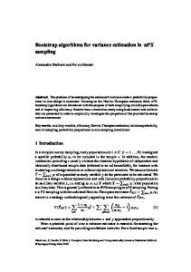
p i ∈ [Np ], Aip−1 is a [Np−1 ]-valued random variable and we write Ap−1 = (A1p−1 , . . . , Ap−1 ) for p ∈ [n] and A = A0:n−1 . A simple algorithmic description of the particle system is given in Algorithm 1. An important and non-standard feature here is that we keep track of a collection of Eve indices E0:n with Ep = N (Ep1 , . . . , Ep p ) for each p, which will be put to use in our variance estimators. We adopt the Eve terminology because Epi represents the index of the time 0 ancestor of ζpi . The fact that Np may vary with p is also atypical, and allows us to address asymptotically optimal particle allocation in Section 6.1. On a first reading, one may wish to assume that N0:n is not time-varying, i.e. cp = 1 so Np = N for all p ∈ {0, . . . , n}. Figure 1 is a graphical representation of a realization of a small particle system.

Algorithm 1. The particle filter. 1. At time 0: for each i ∈ [N0 ], sample ζ0i ∼ M0 (·) and set E0i ← i. 2. At each time p = 1, . . . , n: for each i ∈ [Np ], n o Np−1 1 (a) Sample Aip−1 ∼ C Gp−1 (ζp−1 ), . . . , Gp−1 (ζp−1 ) . Ai

Ai

p−1 p−1 (b) Sample ζpi ∼ Mp (ζp−1 , ·) and set Epi ← Ep−1 .

The particle approximations of ηn and γn are defined respectively, with the convention 1, by the random measures (n−1 ) Y X 1 ηnN = δζni , γnN = ηpN (Gp ) ηnN , Nn p=0

Q−1

p=0

ηpN (Gp ) =

i∈[Nn ]

and we observe that, similar to (2), ηnN = γnN /γnN (1). To simplify presentation, the dependence of γnN and ηnN on c0:n is suppressed from the notation. The following proposition establishes basic properties of the particle approximations, which validate their use. Proposition 1. There exists a map σn2 : L(X ) → [0, ∞) such that for any ϕ ∈ L(X ):

3

ζ01

ζ11

ζ21

ζ31

ζ02

ζ12

ζ22

ζ32

ζ03

ζ13

ζ23

ζ33

ζ04

ζ34

i Figure 1: A particle system with n = 3 and N0:3 = (4, 3, 3, 4). An arrow from ζp−1 to ζpj indicates j j i that the ancestor of ζp is ζp−1 , i.e. Ap−1 = i. In the realization shown, the ancestral indices are A0 = (1, 2, 4), A1 = (2, 1, 2) and A2 = (3, 2, 2, 3), while the Eve indices are E0 = (1, 2, 3, 4), E1 = (1, 2, 4), E2 = (2, 1, 2) and E3 = (2, 1, 1, 2).

 1. E γnN (ϕ) = γn (ϕ), for all N ≥ 1,

 2. γnN (ϕ) → γn (ϕ) almost surely and N var γnN (ϕ)/γn (1) → σn2 (ϕ), h 2 i 3. ηnN (ϕ) → ηn (ϕ) almost surely and N E ηnN (ϕ) − ηn (ϕ) → σn2 (ϕ − ηn (ϕ)).

In the case that the number of particles is constant over time, Np = N , these properties are well known and can be deduced, for example, from various results of Del Moral [2004]. The arguments used to treat the general Np = ⌈cp N ⌉ case are not substantially different, but since they seem not to have been published anywhere in exactly the form we need, we include a proof of Proposition 1 in the supplement.

2.5

A variance estimator

For ϕ ∈ L(X ), consider the quantity VnN (ϕ) = ηnN (ϕ)2 −

n−1 Y p=0

Np Np − 1

!

1 Nn (Nn − 1)

X

ϕ(ζni )ϕ(ζnj ),

(4)

i 6=E j i,j:En n

which is readily computable as a byproduct of Algorithm 1. The following theorem is the first main result of the paper. We state it here to make some of the practical implications of our work accessible to the reader before entering into more technical details; it shows that via (4), the Eve variables Eni can be used to estimate the Monte Carlo errors associated with γnN (ϕ) and ηnN (ϕ). Theorem 1. The following hold for any ϕ ∈ L(X ), with σn2 (·) as in Proposition 1:   1. E γnN (1)2 VnN (ϕ) = var γnN (ϕ) for all N ≥ 1, 2. N VnN (ϕ) → σn2 (ϕ) in probability,

3. N VnN (ϕ − ηnN (ϕ)) → σn2 (ϕ − ηn (ϕ)) in probability. The proof of Theorem 1, given in the appendix, relies on a number of intermediate results concerning moment properties of the particle approximations which we shall develop in the coming sections. Before embarking on this development let us discuss how (4) may be interpreted. Consider random variables ¯ and sample variance X 1 , . . . , X N with sample mean X ¯2 − X

X X 1 1 ¯ 2. (X i − X) X iX j = N (N − 1) N (N − 1) i i6=j

4

(5)

When X 1 , . . . , X N are independent and identically distributed it is of course elementary that (5) ¯ and consistency properties are easily established. Observe the is an unbiased estimator of var(X) resemblance between (4) and the left hand side of (5). Some of the features which distinguish these two expressions, notably the summation over {(i, j) : Eni 6= Enj } and the product term in (4), are a reflection of the dependence between the particles and specific distributional characteristics of Algorithm 1. One of the main difficulties we face is to develop a suitable mathematical perspective from which to describe this dependence and thus establish that (4) does indeed have the properties stated in Theorem 1. It seems natural to ask if (4) can be re-written so as to resemble the right hand side of (5) and thus be interpreted as some kind of sample variance across the population of particles. This motivates the following corollary, using the notation 1 X #in = card{j : Enj = i}, ∆in = i ϕ(ζnj ) − ηnN (ϕ), #n j j:En =i

with the convention ∆in = 0 when #in = 0. Recall from Section 2.3 that in the hidden Markov model and sequential simulation examples γn (1) is respectively the marginal likelihood and ratio of normalizing constants, hence our interest in VnN (ϕ) with specifically ϕ = 1. Corollary 1. In the case that cp = 1 for all p ∈ {0, . . . , n}, 1 X i N VnN (1) = (#n − 1)2 − n + Op (1/N ), N

(6)

i∈[N ]

N VnN (ϕ − ηnN (ϕ)) =

1 X i i 2 (#n ∆n ) + Op (1/N ). N

(7)

i∈[N ]

The proof P is in the supplement. Since i #in = N , the first term on the right hand side of (6) can be interpreted as a sample variance of the #in ’s, reflecting variation in the numbers of time n descendants across the population P of time 0 particles. Since i #in ∆in = 0, the first term on the right hand side of (7) can be interpreted i as a sample P variancej which reflects both variation inNthe #n ’s and the deviations of ithe familial means i −1 j (#n ) =i ϕ(ζn ) from the population mean ηn (ϕ). Note that when n = 0, E0 = i always and j:En V0N (ϕ − η0N (ϕ)) =

X  2 1 ϕ(ζ0i ) − η0N (ϕ) , N0 (N0 − 1) i∈[N0 ]

which is in keeping with ζ0i being independent and identically distributed according to η0 .

3 3.1

Moment properties of the particle approximations Genealogical tracing variables

Our next step is to introduce some auxiliary random variables associated with the genealogical structure of the particle system. These auxiliary variables are introduced only for purposes of analysis: they will assist in deriving and justifying our variance estimators. Given (A, ζ), the first collection of variables, K 1 = (K01 , . . . , Kn1 ), is conditionally distributed as follows: Kn1 is uniformly distributed on [Nn ] and K1

for each p = n − 1, . . . , 0, Kp1 = Ap p+1 . Given (A, ζ) and K 1 , the second collection of variables, K 2 = (K02 , . . . , Kn2 ), is conditionally distributed as follows: Kn2 is uniformly distributed on [Nn ] and K2

N

2 1 6= Kp+1 and Kp2 ∼ C(Gp (ζp1 ), . . . , Gp (ζp p )) if for each p = n − 1, . . . , 0 we have Kp2 = Ap p+1 if Kp+1 2 1 1 Kp+1 = Kp+1 . The interpretation of K is that it traces backwards in time the ancestral lineage of a particle chosen randomly from the population at time n. K 2 is slightly more complicated: it traces backwards in time a sequence of broken ancestral lineages, where breaks in the lineages occur when components of K 1 and K 2 coincide.

5

3.2

Lack-of-bias and second moment of γnN (ϕ)

We now give expressions for the first two moments of γnN (ϕ). n o  K1 Lemma 1. For any ϕ ∈ L(X ), E γnN (1)ϕ(ζn n ) = γn (ϕ) and E γnN (ϕ) = γn (ϕ).

 The proof is in the supplement. This lack-of-bias property E γnN (ϕ) = γn (ϕ) is quite well known and a martingale proof for the Np = N case can be found, for example, in Del Moral [2004, Ch. 9]. In order to present an expression for the second moment of γnN (ϕ), we now introduce a collection of measures on X ⊗2 , denoted {µb : b ∈ Bn } where Bn = {0, 1}n+1 is the set of binary strings of length n + 1. The measures are constructed as follows. For a given b ∈ Bn , let (Xp , Xp′ )0≤p≤n be a Markov chain with state-space X2 , distributed according to the following recipe. If b0 = 0 then X0 ∼ M0 and X0′ ∼ M0 independently, while if b0 = 1 then X0′ = X0 ∼ M0 . Then, for p = 1, . . . , n, if bp = 0 then ′ Xp ∼ Mp (Xp−1 , ·) and Xp′ ∼ Mp (Xp−1 , ·) independently, while if bp = 1 then Xp′ = Xp ∼ Mp (Xp−1 , ·). Letting Eb denote expectation with respect to the law of this Markov chain we then define # " n−1 Y ′ ′ S ∈ X ⊗2 , b ∈ Bn . Gp (Xp )Gp (Xp ) , µb (S) = Eb I {(Xn , Xn ) ∈ S} p=0

n o Qn−1 Similarly to (3) we shall write µb (ϕ) = Eb ϕ(Xn , Xn′ ) p=0 Gp (Xp )Gp (Xp′ ) , for ϕ ∈ L(X ⊗2 ) and b ∈ Bn . Remark 1. Observe that with 0n ∈ Bn denoting the zero string, µ0n (ϕ⊗2 ) = γn (ϕ)2 . Let [N0:n ] = [N0 ] × · · · × [Nn ], and for any b ∈ Bn , I(b) = {(k 1 , k 2 ) ∈ [N0:n ]2 : for each p, kp1 = kp2 ⇐⇒ bp = 1}, which is the set of pairs of [N0:n ]-valued strings which coincide in their p-th coordinate exactly when bp = 1. Lemma 2. For any ϕ ∈ L(X ⊗2 ) and b ∈ Bn , n i Y h  1 2 N 2 Kn Kn 1 2 E I (K , K ) ∈ I(b) γn (1) ϕ(ζn , ζn ) =

p=0

and

(

1 Np

bp  1−bp ) 1 1− µb (ϕ) Np

bp  1−bp n  X Y  N 1 1 2 1− µb (ϕ⊗2 ). E γn (ϕ) = N N p p p=0

(8)

(9)

b∈Bn

The proof of Lemma 2 is in the supplement and uses an argument involving the law of a doubly conditional sequential Monte Carlo algorithm [see also Andrieu et al., 2016]. The identity (9) was first proved by Cérou et al. [2011] in the case where Np = N . Our proof technique is different: we obtain (9) as a consequence of (8). The appearance of K 1 , K 2 in (8) is also central to the justification of our variance estimators below.

3.3

Asymptotic variances

For each p ∈ {0, . . . , n}, we denote by ep ∈ Bn the vector with a 1 in position p and zeros elsewhere. As in Remark 1, 0n denotes the zero string in Bn . The following result builds upon Lemmas 1–2. It shows that a particular subset of the measures {µb : b ∈ Bn }, namely µ0n and {µep : p = 0, . . . , n}, appear in the asymptotic variances.

6

Lemma 3. For any ϕ ∈ L(X ), define vp,n (ϕ) =

µep (ϕ⊗2 ) − µ0n (ϕ⊗2 ) , γn (1)2

p ∈ {0, . . . , n}.

(10)

 Pn Then N var γnN (ϕ)/γn (1) → p=0 c−1 p vp,n (ϕ) and NE

h

n X 2 i → c−1 ηnN (ϕ) − ηn (ϕ) p vp,n (ϕ − ηn (ϕ)).

(11)

p=0

The proof of Lemma 3 is in the supplement. Remark 2. In light of Lemma 3, the map σn2 in Proposition 1 satisfies σn2 (ϕ) =

n X

c−1 p vp,n (ϕ),

ϕ ∈ L(X ).

(12)

p=0

An expression for vp,n (ϕ) in terms of (Mp , Gp )0≤p≤n is obtained by observing that if we define Qp (xp−1 , dxp ) = Gp−1 (xp−1 )Mp (xp−1 , dxp ),

p ∈ {1, . . . , n},

and Qn,n = Id, Qp,n = Qp+1 · · · Qn for p ∈ {0, . . . , n−1}, then µep (ϕ) = γp (Qp,n (ϕ)2 ). In combination with Remark 1, we obtain vp,n (ϕ) =

4 4.1

ηp (Qp,n (ϕ)2 ) γp (1)γp (Qp,n (ϕ)2 ) − ηn (ϕ)2 = − ηn (ϕ)2 . 2 γn (1) ηp Qp,n (1)2

(13)

The estimators Particle approximations of each µb

We now introduce particle approximations of the measures {µb : b ∈ Bn }, from which we shall subsequently derive the variance estimators. For each b ∈ Bn , and ϕ ∈ L(X ⊗2 ) we define " n  1−bp # h  i Y Np K1 K2 bp N γnN (1)2 E I (K 1 , K 2 ) ∈ I(b) ϕ(ζn n , ζn n ) | A, ζ . (14) µb (ϕ) = (Np ) Np − 1 p=0 Recalling from Section 3.1 that given A and ζ, Kn1 and Kn2 are conditionally independent and each uniformly distributed on [Nn ], it follows from (14) that γnN (ϕ)2

= =

1 X ϕ(ζni )ϕ(ζnj ) Nn2 i,j∈[Nn ] i X h  K1 K2 E I (K 1 , K 2 ) ∈ I(b) ϕ(ζn n )ϕ(ζn n ) | A, ζ γnN (1)2

γnN (1)2

b∈Bn

=

X

b∈Bn

(

bp  1−bp n  Y 1 1 1− Np Np p=0

)

⊗2 µN ), b (ϕ

mirroring (9). This identity is complemented by the following result. Theorem 2. For any b ∈ Bn and ϕ ∈ L(X ⊗2 ),  1. E µN b (ϕ) = µb (ϕ) for all N ≥ 1, 7

(15)

2. supN ≥1 N E

h 2 i < ∞ and hence µN µN b (ϕ) → µb (ϕ) in probability. b (ϕ) − µb (ϕ)

The proof of Theorem 2 is in the supplement. Although (14) can be computed in principle from the output of Algorithm 1 without the need for any further simulation, the conditional expectation ⊗2 in (14) involves a summation over all binary strings in I(b), so calculating µN ) in practice may b (ϕ be computationally expensive. Fortunately, relatively simple and computationally efficient expressions ⊗2 are available for µN ) in the cases b = 0n and b = ep , and those are the only ones required to b (ϕ construct our variance estimators.

4.2

Variance estimators

Our next objective is to explain how (4) is related to the measures µN b and to introduce another family of estimators associated with the individual terms in (12). We need the following technical lemma. n o  K1 K2 Lemma 4. The following identity of events holds: En n 6= En n = (K 1 , K 2 ) ∈ I(0n ) .

The proof is in the appendix. Combined with the fact that given (A, ζ), Kn1 , Kn2 are independent and identically distributed according to the uniform distribution on [Nn ], we have i h  X K1 K2 E I (K 1 , K 2 ) ∈ I(0n ) ϕ(ζn n , ζn n ) | A, ζ = Nn−2 ϕ(ζni )ϕ(ζnj ), (16) i 6=E j i,j:En n

and therefore we arrive at the following equivalent of (4), written in terms of µN 0n , VnN (ϕ)

=

ηnN (ϕ)2 −

⊗2 ) µN 0n (ϕ . N 2 γn (1)

(17)

Detailed pseudocode for computing VnN (ϕ) in O(N ) time and space upon running Algorithm 1 is provided in the supplement. Mirroring (10), we now define N vp,n (ϕ) =

⊗2 ⊗2 ) ) − µN µN 0n (ϕ ep (ϕ

γnN (1)2

,

p ∈ {0, . . . , n},

vnN (ϕ) =

n X

N c−1 p vp,n (ϕ).

p=0

N Detailed pseudocode for computing each vp,n (ϕ) and vnN (ϕ) with time and space complexity in O(N n) time upon running Algorithm 1 is provided in the supplement. The time complexity is the same as that of running Algorithm 1, but the space complexity is larger. Empirically, we have found that N VnN (ϕ) is very similar to vnN (ϕ) as an estimator of σn2 (ϕ) when N is large enough that they are both accurate, and hence may be preferable due to its reduced space complexity.

Theorem 3. For any ϕ ∈ L(X ),  N (ϕ) = γn (1)2 vp,n (ϕ) for all N ≥ 1, 1. E γnN (1)2 vp,n

N N 2. vp,n (ϕ) → vp,n (ϕ) and vp,n (ϕ − ηnN (ϕ)) → vp,n (ϕ − ηn (ϕ)), both in probability,  3. E γnN (1)2 vnN (ϕ) = γn (1)2 σn2 (ϕ) for all N ≥ 1 and vnN (ϕ) → σn2 (ϕ) in probability.

5

Estimators for updated measures

In some applications there is interest in approximating the updated measures: ˆ γˆn (S) , S ∈ X. Gn (x)γn (dx), ηˆn (S) = γˆn (S) = γˆn (1) S 8

In the hidden Markov model setting described in Section 2.2, e.g., ηˆn is the conditional distribution of Xn given y0 , . . . , yn , that is ηˆn is a filtering distribution, while ηn is a predictive distribution. The updated particle approximations are defined by ˆ γˆ N (S) , S ∈ X, γˆnN (S) = Gn (x)γnN (dx), ηˆnN (S) = nN γˆn (1) S and we now define their variance estimators. To facilitate this task, we consider a fixed ϕ ∈ L(X ), and define ϕ(x) ˆ = Gn (x)ϕ(x). The following relationships can then be deduced: γˆn (ϕ) ≡ γn (ϕ), ˆ ηˆn (ϕ) ≡ ηn (ϕ)/η ˆ n (Gn ), γˆnN (ϕ) ≡ γnN (ϕ) ˆ and ηˆnN (ϕ) ≡ ηnN (ϕ)/η ˆ nN (Gn ). We define analogues of σn2 and vp,n for the updated particle approximations as  σ ˆn2 (ϕ) = lim N var γˆnN (ϕ)/ˆ γn (1) , N →∞

vˆp,n (ϕ) =

vp,n (ϕ) ˆ , ηn (Gn )2

and the proposition below is a counterpart to Proposition 1 and Lemma 3. Proposition 2. For any ϕ ∈ L(X ), 1. γˆnN (ϕ) → γˆn (ϕ) almost surely and σ ˆn2 (ϕ) =

n X

c−1 ˆp,n (ϕ), p v

p=0

2. ηˆnN (ϕ) → ηˆn (ϕ) almost surely and N E

h

2 i →σ ˆn2 (ϕ − ηˆn (ϕ)). ηˆnN (ϕ) − ηˆn (ϕ)

The proofs of Proposition 2, and Theorems 4–5 below can be found in the supplement. Proposition 2 implies the relationship σ ˆn2 (ϕ) = σn2 (ϕ)/η ˆ n (Gn )2 . The corresponding estimates of the variance, asymptotic variance and the terms therein are now obtained and analogues of Theorems 1 and 3 folN N low straightforwardly. Below we write the estimators VˆnN , vˆp,n etc. in terms of VnN , ηnN and vp,n to N N emphasize that the same algorithms can be used to compute them, just as γˆn (ϕ) and ηˆn (ϕ) can be ˆ nN (Gn ), respectively. computed as γnN (ϕ) ˆ and ηnN (ϕ)/η Theorem 4. For any ϕ ∈ L(X ), with VˆnN (ϕ) = VnN (ϕ)/η ˆ nN (Gn )2 , n o  1. E γˆnN (1)2 VˆnN (ϕ) = var γˆnN (ϕ) for all N ≥ 1,

(18)

2. N VˆnN (ϕ) → σ ˆn2 (ϕ) in probability,

3. N VˆnN (ϕ − ηˆnN (ϕ)) → σ ˆn2 (ϕ − ηˆn (ϕ)) in probability. Remark 3. It follows from (4), (17), (18) and simple manipulations that  #2 "P j j X ˆnN (ϕ) j N VˆnN (ϕ − ηˆnN (ϕ)) =i Gn (ζn ) ϕ(ζn ) − η j∈[Nn ]:En Q  =N , P j n Np j∈[Nn ] Gn (ζn ) i∈[N ] p=0 Np −1

0

the right hand side of which is, in the case where N is not time-varying, precisely the estimator in Equation 2.9 of Chan and Lai [2013].

Theorem 5. For any ϕ ∈ L(X ), with N N vˆp,n (ϕ) = vp,n (ϕ)/η ˆ nN (Gn )2 ,

vˆnN (ϕ) =

n X

N c−1 ˆp,n (ϕ), p v

p=0

N 1. E γˆnN (1)2 vˆp,n (ϕ) = γˆn (1)2 vˆp,n (ϕ) for all N ≥ 1, 

N N 2. vˆp,n (ϕ) → vˆp,n (ϕ) and vˆp,n (ϕ − ηˆnN (ϕ)) → vˆp,n (ϕ − ηˆn (ϕ)), both in probability,  N 2 N 3. E γˆn (1) vˆn (ϕ) = γˆn (1)2 σ ˆn2 (ϕ) for all N ≥ 1 and vˆnN (ϕ) → σ ˆn2 (ϕ) in probability.

9

6

Use of the estimators to tune the particle filter

The variance estimators we have proposed can of course be applied directly to report estimates of Monte Carlo error alongside particle approximations. Estimates of quantities such as vp,n (ϕ) may also aid algorithm and design. We provide here two simple examples of adaptive methods to illustrate this, firstly concerning how to improve performance by allowing particle numbers to vary over time, and secondly concerning how to choose particle numbers so as to achieve some user-defined performance criterion. To simplify presentation, we focus on performance in estimating γnN (ϕ), the ideas can easily be modified easily to deal instead with ηnN (ϕ), γˆnN (ϕ) or ηˆnN (ϕ).

6.1

Asymptotically optimal allocation

The following well known result is closely related to Neyman’s optimal allocation in stratified random sampling [Tschuprow, 1923, Neyman, 1934]. A short proof using Jensen’s inequality can be found in Glasserman [2004, Section 4.3]. Pn Lemma 5. Let a0 , . . . , an ≥ 0. The function (c0 , . . . , cn ) 7→ p=0 c−1 p ap is minimized, subject to the Pn 1/2 2 −1 constraints minp cp > 0 and p=0 cp = n + 1, at (n + 1) kak2 when cp ∝ ap .

As a consequence, we can in principle minimize σn2 (ϕ) by choosing cp ∝ vp,n (ϕ)1/2 . An approximation of this optimal allocation can be obtained by the following two-stage procedure. First  Nrun a particle N filter with Np = N to obtain the estimates vp,n (ϕ) and then define c0:n by cp = max vp,n (ϕ), g(N ) , where g is some positive but decreasing function with limN →∞ g(N ) = 0. Then run a second particle filter with each Np = ⌈cp N ⌉, and report the quantities of interest, e.g., γnN (ϕ). The function gPis chosen to ensure cp > 0 and that for large N we permit small values of cp . The quantity Pn that n N −1 N p=0 vp,n (ϕ)/( p=0 cp vp,n (ϕ)), obtained from the first run, is an indication of the improvement in variance obtained by using the new allocation. Approximately optimal allocation has previously been addressed by Bhadra and Ionides [2016], who introduced a meta-model to approximate the distribution of the Monte Carlo error associated with log γnN (1) in terms of an autoregressive process, the objective function to be minimized then being the variance under this meta-model. They provide only empirical evidence for the fit of their meta-model, whereas our approach targets the true asymptotic variance σn2 (ϕ) directly.

6.2

An adaptive particle filter

Monte Carlo errors of particle filter approximations can be sensitive to N , and an adequate value of N to achieve a given error may not be known a priori. The following procedure increases N until VnN (ϕ) is in a given interval. Consider the case where we wish to estimate γn (ϕ). Given an initial number of particles N (0) and a threshold δ > 0, one can run successive particle filters, doubling the number of particles each time, (τ ) until the associated random variable VnN (ϕ) ∈ [0, δ]. Finally, one runs a final particle filter with (τ ) N particles, and returns the estimate of interest. We provide empirical evidence in Section 7 that this procedure can be effective in some applications.

7

Applications and illustrations

In this section we demonstrate the empirical performance of the estimators we have proposed in three examples. Our numerical results mostly address the accuracy of our estimators of the asymptotic variance σn2 (ϕ), the individual terms vp,n (ϕ), and the effectiveness of the applications described in Section 6 with the test functions ϕ ≡ 1 and ϕ = Id, the identity function. Where the results for later examples are qualitatively similar to those of the first, the corresponding figures can be found in the supplement. 10

Asymptotic variance

Asymptotic variance

0.8

300

200

10

12

14

log2(N)

16

0.6

0.4

0.2

10

12

log2(N)

14

16

N (Id) (b) ϕ = Id − ηˆn

(a) ϕ ≡ 1

Asymptotic variance terms

Figure 2: Estimated asymptotic variances N VˆnN (ϕ) (dots and error bars for the mean ± one standard deviation from 104 replicates) against log2 N for the linear Gaussian example. The horizontal lines correspond to the true asymptotic variances. The sample variances of γˆnN (1)/ˆ γn (1) and ηˆnN (Id), scaled by N , were close to their asymptotic variances.

60

40

20

0 0

25

50

75

100

p N Figure 3: Plot of vˆp,n (1) (dots and error bars for the mean ± one standard deviation from 104 replicates) and vˆp,n (1) (crosses) at each p ∈ {0, . . . , n} for the Linear Gaussian example, with N = 105 .

7.1

Linear Gaussian hidden Markov model

This model is specified by M0 (·) = N (·; 0, 1), Mp (xp−1 , ·) = N (·; 0.9xp−1 , 1) and Gp (xp ) = N (yp ; xp , 1). The measures ηˆn and γˆn are available in closed form via the Kalman filter, and for suitable ϕ the quantities vˆp,n (ϕ) etc. can be computed exactly, allowing us to assess the accuracy of our estimators. We used a synthetic dataset, simulated according to the model with n = 99. A Monte Carlo study with 104 replicates of VˆnN (ϕ) for each value of N and cp ≡ 1 was used to measure the accuracy of the ˆn2 (1) = 295.206 estimate N VˆnN (ϕ) as N grows; results are displayed in Figure 2 and for this data σ 2 N N ˆ and σ ˆn (Id − ηˆn (Id)) ≈ 0.58. The estimates vˆn (ϕ) differed very little from N Vn (ϕ), and so are not N shown. We then tested the accuracy of the estimates vˆp,n (1); results are displayed in Figure 3. The N N estimates vˆp,n (Id − ηˆn (Id)) are very close to 0 for p < 95 and with values (0.0017, 0.012, 0.082, 0.48) for p ∈ {96, 97, 98, 99}; this behaviour is in keeping with time-uniform bounds on asymptotic variances obtained by Whiteley [2013], see also references therein. We also compared a constant N particle filter, the asymptotically optimal particle filter where the asymptotically optimal allocation is computed exactly, and its approximation described in Section 6.1 for different values of N using a Monte Carlo study with 104 replicates. We took g(N ) = 2/ log2 N in defining the approximation, and the results in Figure 4a indicate that indeed the approximation reduces the variance. The improvement is fairly modest for this particular model, and indeed the exact asymptotic variances associated with the constant N and asymptotically optimal particle filters differ by less than a factor of 2. In contrast, Figure 4b shows that the improvement can be fairly dramatic 11

log2(sample variance)

log2(sample variance)

−2

−4

−6

10

11

12

13

log2(N)

14

2 0 −2 −4 −6

15

10

(a)

11

12

13

log2(N)

14

15

(b)

Figure 4: Logarithmic plots of the sample variance across 104 replicates of γnN (1)/γn (1) against N for the linear Gaussian example, using a constant N particle filter (dotted), the approximation to the asymptotically optimal particle filter (dot-dash), and the asymptotically optimal particle filter (solid). In Figure 4b, the observation sequence is yp = 0 for p ∈ {0, . . . , 99} \ {49} and y49 = 8. 15

−2

14

−3

13

log2(N)

log2(sample variance)

−1

−4

12

−5 11 −6 10 −6

−4

log2(δ)

−2

−6

(a)

−4

log2(δ)

−2

(b)

Figure 5: Logarithmic plots for the simple adaptive N particle filter estimates of γˆn (1) for the linear Gaussian example. Figure (a) plots the sample variance of γˆnN (1)/ˆ γn (1) against δ, with the straight line y = x. Figure (b) plots N against δ, where N is the average number of particles used by the final particle filter. in the presence of outlying observations; the improvement in variance there is by a factor of around 40. Finally, we tested the adaptive particle filter described in Section 6.2 using 103 replicates for each value of δ; results are displayed in Figure 5, and indicate that the estimates of γˆn (1) are close to their prescribed thresholds.

7.2

Stochastic volatility hidden Markov model

 A stochastic volatility model is defined by M0 (·) = N · ; 0, σ 2 /(1 − ρ2 ) , Mp (xp−1 , ·) = N ( · ; ρxp−1 , σ 2 ) and Gp (xp ) = N (yp ; 0, β 2 exp(xp )). We used the pound/dollar daily exchange rates for 100 consecutive weekdays ending on 28th June, 1985, a subset of the well-known dataset analyzed in Harvey, Ruiz and Shephard (1994). Our results are obtained by choosing the parameters (ρ, σ, β) = (0.95, 0.25, 0.5). We provide in the supplement plots of the accuracy of the estimate N VˆnN (ϕ) as N grows using 104 replicates for each value of N ; the asymptotic variances σ ˆn2 (1) and σ ˆn2 (Id − ηˆn (Id)) are estimated as being approximately 354 and 1.31 respectively. In the supplement we plot the estimates of vˆp,n (ϕ). We found modest improvement for the approximation of the asymptotically optimal particle filter, as one could infer from the estimated vˆp,n (ϕ). For the simple adaptive N particle filter, results are provided in the supplement, and indicate that the estimates of γˆn (1) are close to their prescribed thresholds.

12

0.1

90

60

30

0

0.0 0

3

6

9

(a) ϕ ≡ 1, k = 10

2.0

1.5

1.0

0.5

300

200

100

0.0 0

p

Asymptotic variance terms

0.2

Asymptotic variance terms

Asymptotic variance terms

Asymptotic variance terms

0.3

3

6

9

0

p

3

6

9

0

3

p

(b) ϕ = Id − ηn (Id), k = 10

(c) ϕ ≡ 1, k = 1

6

9

p

(d) ϕ = Id − ηn (Id), k = 1

N Figure 6: Plot of vp,n (ϕ) (dots and error bars for the mean ± one standard deviation) at each p ∈ {0, . . . , n} with k = 10 iterations (a)–(b) and k = 1 iteration (c)–(d) for each Markov kernel in the SMC sampler example and N = 105 .

7.3

An SMC sampler

We consider a sequential simulation problem, as described in Section 2.3, with X = R, π ¯0 (x) = N (0, 102 ) and π ¯1 (x) = 0.3N (x; −10, 0.12) + 0.7N (x; 10, 0.22). The distribution π1 is bi-modal with well-separated modes. With n = 11, and the sequence of tempering parameters β0:n = (0, 0.0005, 0.001, 0.0025, 0.005, 0.01, 0.025, 0.05, 0.1, 0.25, 0.5, 1), we let each Markov kernel Mp , p ∈ {1, . . . , n} be an ηp -invariant random walk Metropolis kernel iterated k = 10 times with proposal variance τp2 , where τ1:n = (10, 9, 8, 7, 6, 5, 4, 3, 2, 1, 1). One striking difference between the estimates for this model and those for the hidden Markov models above is that the asymptotic variance σn2 (Id − ηn (Id)) ≈ 822 is considerably larger than σn2 (1) ≈ 2.1; the variability of the estimates N VnN (ϕ) is shown in the supplement. Inspection of the estimates of vp,n (ϕ) in Figures 6 allows us to investigate both this difference and the dependence of vp,n (ϕ) on k in greater detail. In Figure 6(a)–(b) we can see that while vp,n (1) is small for all p, the values of vp,n (Id − ηn (Id)) are larger for large p than for small p; this could be due to the inability of the Metropolis kernels (Mq )q≥p to mix well due to the separation of the modes in (ηq )q≥p when p is large. In Figure 6(c)–(d), k = 1, that is each MP consists of only a single iterate of a Metropolis kernel, and we see that the values of vp,n (ϕ) associated with small p are much larger than when k = 10, indicating that the larger number of iterates does improve the asymptotic variance of the particle approximations. However, the impact on vp,n (ϕ) is less pronounced for large p. Results for the simple adaptive N particle filter approximating ηn (Id) are provided in the supplement, which again show that the estimates are close to their prescribed thresholds.

8 8.1

Discussion Alternatives to the bootstrap particle filter

In the hidden Markov model examples above, we have constructed the Feynman–Kac measures taking M0 , . . . , Mn to be the initial distribution and transition probabilities of the latent process and defining G0 , . . . , Gn to incorporate the realized observations. This is only one, albeit important, way to construct particle approximations of ηn , and the algorithm itself is usually referred to as the bootstrap particle filter. Alternative specifications of (Mp , Gp )0≤p≤n lead to different Feynman-Kac models, as discussed in Del Moral [2004, Section 2.4.2], and the variance estimators introduced here are applicable to these models as well. 13

Asymptotic variance terms

5 4 3 2 1 0 0

25

50

75

100

p N Figure 7: Plot of vˇp,n (1) (dots and error bars for the mean ± one standard deviation) and vˇp,n (1) (crosses) at each p ∈ {0, . . . , n} in the Linear Gaussian example.

One particular specification corresponds to the “fully adapted” auxiliary particle filter of Pitt and Shephard ˇ 0 (dx0 ) = M0 (dx0 )G0 (x0 )/M0 (G0 ), [1999], as discussed by Doucet and Johansen [2008]. Specifically, we define M and ˇ p (xp−1 , dxp ) = Mp (xp−1 , dxp )Gp (xp ) , M p ∈ [n], Mp (Gp )(xp−1 ) ˇ 0 (x0 ) = M0 (G0 )M1 (G1 )(x0 ) and G ˇ p (xp ) = Mp+1 (Gp+1 )(xp ), p ≥ 1. If we denote by γˇn and then G ˇ p, G ˇ p )0≤p≤n , we obtain γˇn = γˆn and ηˇn = ηˆn . and ηˇn the Feynman–Kac measures associated with (M Moreover, the variances of γˇnN (ϕ) and ηˇnN (ϕ) are often smaller than the variances of γˆnN (ϕ) and ηˆnN (ϕ). In Figure 7, we plot the corresponding vˇp,n (1) and their approximations for the same linear Gaussian example in Section 7.1. Here, the asymptotic variance of γˇnN (1)/ˇ γn (1) is 40.718, more than 7 times smaller than σ ˆn2 (1).

8.2

Estimators based on i.i.d. replicates

It is clearly possible to estimate consistently the variance of γnN (ϕ)/γn (1) by using i.i.d. replicates of γnN . Such estimates necessarily entail simulation of multiple particle filters. We now compare the accuracy of such estimates with those based on i.i.d. replicates of VnN (ϕ). For somePϕ ∈ L(X ) and B ∈ N, let N N N γn,i (ϕ) and Vn,i (ϕ) be i.i.d. replicates for i ∈ [B], and define M = N −1 i∈[B] γn,i (1). A standard  N −1 N estimate of var γn (ϕ)/γn (1) is obtained by calculating the sample variance of {M γn,i (ϕ); i ∈ [B]}.   Noting the lack-of-bias of γnN (1)2 VnN (ϕ), an alternative estimate of var γnN (ϕ)/γn (1) can be obtained P N N (1)]2 Vn,i (ϕ). Both these estimates can be seen as ratios of simple Monte Carlo as B1 i∈[B] [M −1 γn,i  N estimates of var γn (ϕ) and γn (1)2 , and are therefore consistent as B → ∞. We show in Figure 8 a comparison between these estimates for the three models discussed in Section 7 with N = 103 and ϕ ≡ 1, and we can see that the alternative estimate based on VˆnN (1) is empirically more accurate for these examples.

8.3

Final remarks

The particular approximations developed here provide a natural way to estimate the terms appearing in the non-asymptotic second moment expression (9). To the best of our knowledge, we have also provided the first generally applicable, consistent estimators of vp,n (ϕ). The expression (9) does not apply to particle approximations with resampling schemes other than multinomial, and one possible avenue of future research is to investigate estimators in these other settings. Whilst we have emphasized variances and asymptotic variances, the measures µb also appear in expressions which describe propagation of chaos properties of the particle system. For instance, in the situation Np ≡ N , the asymptotic bias

14

0.6

0.5

0.3

0.2

Variance estimate

Variance estimate

Variance estimate

0.5 0.4

0.4 0.3 0.2

0.003

0.002

0.001

0.1

0.1 5

10

20

50

100

5

10

20

B

50

100

5

B

10

20

50

100

B

  Figure 8: Plot of the standard estimate of var γˆnN (ϕ)/ˆ γn (1) (gray dots and error bars) and the alternative estimate using VˆnN (1) (black crosses and error bars) against B in (left to right) the examples of Sections 7.1–7.3. formula of Del Moral et al. [2007, p.7.] can be expressed as n−1 n−1 X µep {1 ⊗ (ϕ − ηn (ϕ))} X ηp {Qp,n (1)Qp,n (ϕ − ηn (ϕ))}  ≡ − , N E ηnN (ϕ) − ηn (ϕ) → − 2 ηp Qp,n (1) γn (1)2 p=0 p=0 N which could be consistently estimated by replacing µep and γn (1) by µN ep and γn (1). Finally, the technique used in the proof of Lemma 2 can be generalized to obtain expressions for arbitrary positive integer moments of γnN (ϕ).

Supplementary Material The supplementary material at http://www.warwick.ac.uk/alee/vestpf_supp.pdf includes algorithms for efficient computation of the variance estimators, and proofs of Corollary 1, Lemmas 1–3, Propositions 1–2, and Theorems 2, 4 and 5.

Appendix Proof of Theorem 1. Throughout the proof, → denotes convergence in probability. For part 1., the fact µ0n (ϕ⊗2 ) = γn (ϕ)2 and Theorem 2 together give     ⊗2 ) = E γnN (ϕ)2 − γn (ϕ)2 = var γnN (ϕ) . E γnN (1)2 VnN (ϕ) = E γnN (ϕ)2 − µN 0n (ϕ

⊗2 For part 2., combining the identity (15), µN ) → µb (ϕ⊗2 ) by Theorem 2, and the fact that for any b (ϕ 1−bp Qn  1 bp  b ∈ Bn other than 0n and e0 , . . . , en , p=0 Np 1 − N1p is in O(N −2 ), we obtain

γnN (ϕ)2

−

⊗2 ) µN 0n (ϕ

=

(

n ⊗2 ⊗2 X ) ) − µN µN 0n (ϕ ep (ϕ

⌈cp N ⌉

p=0

)

+ Op (N −2 ).

(19)

Also noting that by Proposition 1 γnN (1)2 → γn (1)2 , from (10) that γn (1)2 vp,n (ϕ) = µep (ϕ⊗2 ) − ⊗2 ) → µb (ϕ⊗2 ), we then have µ0n (ϕ⊗2 ) and again using µN b (ϕ N VnN (ϕ) =

n X vp,n (ϕ) N  N ⊗2 2 N (ϕ ) → γ (ϕ) − µ = σn2 (ϕ). n 0 n γnN (1)2 c p p=0

15

(20)

For part 3., first note that by Theorem 2 and Proposition 1, for any b ∈ Bn , N ⊗2 µN ) b ([ϕ − ηn (ϕ)]

⊗2 N N 2 N ⊗2 = µN ) − ηnN (ϕ)[µN ) b (ϕ b (ϕ ⊗ 1) + µb (1 ⊗ ϕ)] + ηn (ϕ) µb (1 → µb ([ϕ − ηn (ϕ)]⊗2 ),

from which it follows that (19) also holds with ϕ replaced by ϕ − ηnN (ϕ), and then N VnN (ϕ − ηnN (ϕ)) →

n X vp,n (ϕ − ηn (ϕ))

cp

p=0

= σn2 (ϕ − ηn (ϕ)),

similarly to (20). Bi

p i i Proof of Lemma 4. For i ∈ [Nn ] define Bn−1 = Ain−1 and Bp−1 = Ap−1 for p ∈ [n − 1]. Since in

Ai

p−1 for all p ∈ [n], i ∈ [Np ] , a simple inductive argument then shows that Algorithm 1, Epi = Ep−1

Bi

Eni = Ep p ,

p ∈ {0, . . . , n}, i ∈ [Nn ]. K1

(21)

K2

We shall now prove (K 1 , K 2 ) ∈ I(0n ) ⇒ En n 6= En n . Recall from Section 3.1 that when (K 1 , K 2 ) ∈ Kp1

Kp2

1 Kn

1 2 I(0n ), we have Ap−1 = Kp−1 6= Kp−1 = Ap−1 for all p ∈ [n], hence B0

K2

= K01 6= K02 = B0 n . Applying Bi

(21) with p = 0 and using the fact that in Algorithm 1, E0i = i for all i ∈ [Nn ], we have Eni = E0 0 = B0i , K1

1 Kn

hence En n = B0

2 Kn

6= B0

K2

K1

K2

K1

K2

= En n as required. It remains to prove (K 1 , K 2 ) ∈ / I(0n ) ⇒ En n = En n .

Assuming (K 1 , K 2 ) ∈ / I(0n ), consider τ = max{p : Kp1 = Kp2 }. If τ = n then clearly En n = En n , 1 Kn

so suppose τ < n. It follows from Section 3.1 that Bτ 1 Kn

i = Kn1 , Kn2 in (21) gives En

2 Kn

K2

= Kτ1 = Kτ2 = Bτ n , so taking p = τ and

= En .

Proof of Theorem 3. For part 1., Theorem 2 gives o n  ⊗2 ⊗2 N ) = µep (ϕ⊗2 ) − µ0n (ϕ⊗2 ) = γn (1)2 vp,n (ϕ). ) − µN E γnN (1)2 vp,n (ϕ) = E µN 0n (ϕ ep (ϕ

⊗2 )− For the remainder of the proof, → denotes convergence in probability. For part 2., µN ep (ϕ ⊗2 2 N N 2 2 N µ0n (ϕ ) → γn (1) vp,n (ϕ) by Theorem 2, and γn (1) → γn (1) by Proposition 1, so vp,n (ϕ) = i h N ⊗2 ⊗2 ⊗2 N ) → (ϕ ) /γnN (1)2 → vp,n (ϕ); as in the proof of Theorem 1, µN (ϕ ) − µ µN 0n ep b ([ϕ − ηn (ϕ)]

N µb ([ϕ − ηn (ϕ)]⊗2 ) gives vp,n (ϕ − ηnN (ϕ)) → vp,n (ϕ − ηn (ϕ)). Part 3. follows from parts 1. and 2.

References C. Andrieu, A. Lee, and M. Vihola. Uniform ergodicity of the iterated conditional SMC and geometric ergodicity of particle Gibbs samplers. Bernoulli, 2016. , to appear. A. Bhadra and E. L. Ionides. Adaptive particle allocation in iterated sequential Monte Carlo via approximating meta-models. Stat. Comput., 26(1):393–407, 2016. F. Cérou, P. Del Moral, and A. Guyader. A nonasymptotic theorem for unnormalized Feynman–Kac particle models. Ann. Inst. H. Poincaré Probab. Statist., 47(3):629–649, 2011. H. P. Chan and T. L. Lai. A general theory of particle filters in hidden Markov models and some applications. Ann. Statist., 41(6):2877–2904, 2013. N. Chopin. Central limit theorem for sequential Monte Carlo methods and its application to Bayesian inference. Ann. Statist., 32(6):2385–2411, 2004. 16

P. Del Moral. Feynman-Kac formulae: genealogical and interacting particle systems with applications. Springer Verlag, 2004. P. Del Moral and A. Guionnet. Central limit theorem for nonlinear filtering and interacting particle systems. Ann. Appl. Probab., 9(2):275–297, 1999. P. Del Moral and L. Miclo. Genealogies and increasing propagation of chaos for Feynman-Kac and genetic models. Ann. Appl. Probab., 11(4):1166–1198, 2001. P. Del Moral, A. Doucet, and A. Jasra. Sequential Monte Carlo samplers. J. R. Stat. Soc. Ser. B Stat. Methodol., 68(3):411–436, 2006. P. Del Moral, A. Doucet, and G. W. Peters. Sharp propagation of chaos estimates for Feynman-Kac particle models. Theory Probab. Appl., 51(3):459–485, 2007. R. Douc and E. Moulines. Limit theorems for weighted samples with applications to sequential Monte Carlo methods. Ann. Statist., 36(5):2344–2376, 2008. R. Douc, A. Guillin, and J. Najim. Moderate deviations for particle filtering. Ann. Appl. Probab., 15 (1B):587–614, 2005. A. Doucet and A. M. Johansen. A tutorial on particle filtering and smoothing: fifteen years later. In D. Crisan and B. Rozovsky, editors, Handbook of Nonlinear Filtering. Oxford University Press, 2008. P. Glasserman. Monte Carlo methods in financial engineering. Springer Science & Business Media, 2004. H. Künsch. Recursive Monte Carlo filters: algorithms and theoretical analysis. Ann. Statist., 33(5): 1983–2021, 2005. J. Neyman. On the two different aspects of the representative method: the method of stratified sampling and the method of purposive selection. J. Roy. Statist. Soc., 97(4):558–625, 1934. M. K. Pitt and N. Shephard. Filtering via simulation: auxiliary particle filters. J. Amer. Statist. Assoc., 94(446):590–599, 1999. A. A. Tschuprow. On the mathematical expectation of the moments of frequency distributions in the case of correlated observations. Metron, 2:461–493, 646–683, 1923. N. Whiteley. Stability properties of some particle filters. Ann. Appl. Prob., 23(6):2500–2537, 2013.

17