Such an estimate of say e.g. a position and velocity of an object ... In modern Bayesian estimation theory and more specifically in particle filtering, see ... As already mentioned, in certain applications, e.g. tracking of closely spaced objects, ... The particle filter based MAP estimator for non-linear dynamical systems has first ...
Particle Filter Based MAP estimation for jump Markov systems∗ Yvo Boers†‡ and Hans Driessen Thales Nederland B.V. Arunabha Bagchi Department of Applied Mathematics University of Twente
Abstract In this paper we will provide methods to calculate different types of Maximum A Posteriori (MAP) estimators for jump Markov systems. The MAP estimators that will be provided are calculated on the basis of a running Particle Filter (PF). Furthermore, we will provide convergence results for these approximate, or particle based estimators. We will show that the approximate estimators convergence in distribution to the true MAP estimator values. Additionally, we will provide an example based on tracking closely spaced objects in a binary sensor network to illustrate some of the results and their applicability.
1
Introduction
The focus of this paper is point estimators for stochastic dynamical systems. The application area of this topic is naturally very wide. The scope covers all sorts of fields, such as engineering or finance. In fact, any problem that can be formulated as a dynamical system on which measurements are performed falls in the application area. The process of inferring information on the state of such a system based on measurements is called filtering. Point estimators are most commonly used in filtering. This means that entire a posteriori information obtained in the filtering process is captured in one single value. Such an estimate of say e.g. a position and velocity of an object ia called a point estimate. Examples of popular point estimators are the minimum variance (MV) estimator or the maximum a posteriori (MAP) estimator. It is well known that in case of linear and Gaussian systems, for which the a posteriori densities are Gaussian, the two coincide. However, for general, non-linear and/or non-Gaussian systems they generally do not coincide. An illustration of this is provided in figure 1. ∗ This
paper has been presented in a very preliminary version at the FUSION 2009 conference Author ‡ Yvo Boers also holds a part time position as an NWO-Casimir fellow at the Department of Applied Mathematics at the University of Twente, the Netherlands † Corresponding
1
Comparison of MMSE and MAP estimates multimodal probability density MMSE MAP
0.5
pdf of X
0.4
0.3
0.2
0.1
0
−6
−4
−2
0
2
4
6
X
Figure 1: Multi modal a posteriori probability density with corresponding MMSE and MAP estimates In modern Bayesian estimation theory and more specifically in particle filtering, see e.g. [1], one might argue or question: why concentrate on the topic of point estimation at all ? Especially when the entire a posteriori density is provided anyway, e.g. by means of the particles of a running particle filter. Because it is well known that this a posteriori density is the maximum of information that can be obtained. The answer is very simple: because a lot of practical and operational applications require a point estimate. Moreover, it might be far from trivial to give an interpretation of the entire a posteriori density or the particle cloud. For example, in the case of target tracking, when the filter describes one single target, an interpretation might be not that difficult. However, when the filter describes a multi-target setting, possibly including a description of the number of targets as well, it is far from trivial to provide a good interpretation. Having said all this, we do emphasize that in the scope of this paper the entire underlying description, i.e. the a posteriori probability density, is maintained by a running particle filter. Thus, the MAP estimates provided in this paper are for output reasons only and do not comprise the running particle filter in any way whatsoever. As already mentioned, in certain applications, e.g. tracking of closely spaced objects, see [2] and [3], the MAP estimator can be very useful. Consequently, in [2] it has been shown quantitatively that for the application at hand the MAP estimator is superior to the MV estimator. In general, we can say that for non-linear and/or non-Gaussian systems MAP estimation is a useful alternative for MV estimation. Some other applications, in which multi-modality naturally arises, are terrain aided navigation, see e.g. [4] and figure 2, and tracking in binary sensor networks, see e.g. [5] and figure 3. For these two applications the multi-modality of the a posteriori density is clearly displayed through the particle clouds. However, there are undoubtedly many more applications that will lead to multi-modality of the a posteriori probability density. 2
Figure 2: Terrain navigation example - Particle representation of a posteriori probability density The particle filter based MAP estimator for non-linear dynamical systems has first been presented in [6]. In [6] and [7] it has been shown that based on a running particle filter the MAP estimator can be calculated. Moreover, explicit formulas and an algorithm for calculating this PF based MAP estimator have been provided. Previous to [6] and [7] the particle filter based MAP estimator has sometimes been erroneously thought to be equal to the particle with the highest weight. This idea has been proven wrong in [6] and [7] as well as in the excellent survey article [8]. In [6] and [7] correct analytical expressions and algorithms to calculate the true MAP estimator, based on a running particle filter, have been provided. Furthermore, it has been proven in [6] and [7] that the particle based MAP estimator converges to the true MAP estimator. It is good to note that such a proof does not exist for the regularly used MV estimator, see also [9]. Recently, see [10], for the MV estimator convergence has been proven, although it has been at the cost of additional assumptions on the problem at hand. Also, the earlier work [11] should not be left unmentioned. In this paper a particle based MAP estimator for the whole sequence or trajectory has been presented. Thus, the maximum of p(s0 , s1 , . . . , sk | Zk ) is approximated. The result of this procedure is a maximizing sequence: sˆ0:k . This sequence MAP estimator is obtained by employing a Viterbi optimization at every time step. The complexity of the problem in [11] naturally grows with the time horizon k. In this paper the focus is to obtain a MAP estimate for the current state only. As a result, we are interested in the MAP estimate associated with the filtering density p(sk | Zk ). We also stress the fact that the MAP estimate of the filtering density is not necessarily the same as taking the k th
3
80
70
60
y (m)
50
40
30
20
10
0
0
10
20
30
40 x (m)
50
60
70
80
Figure 3: Particle description of a posteriori probability density element of the sequence MAP estimator. Especially in the case of multi-modal a posteriori densities these estimates do not have to coincide at all. We will show this in the small illustrative example below.
0.08
maximum of the 2D Gaussian sum pdf
pdf value
0.06
0.04
0.02
0 40
40 30
30 20
20 S1
10
10 0
0
S2
Figure 4: 2D joint Gaussian sum probability density function
4
0.06 24 0.055 22 0.05
20
0.045
18
s1
16
maximizing argument for the 1D, marginalized Gaussian sum pdf
14
0.04 0.035
maximizing argument for the 2D Gaussian sum pdf
12
0.03
10 0.025 8 0.02
6
0.015
4 16
17
18
19
20 s
21
22
23
0.01
24
2
Figure 5: Contour of the 2D joint Gaussian sum probability density function
0.25
pdf value
0.2
Maximum of the marginalized pdf
0.15
0.1
Maximizing argument of the marginalized pdf 0.05
0
0
5
10
15
20
25
30
35
40
s1
Figure 6: Marginalized Gaussian sum probability density function Consider a two dimensional Gaussian sum density, defined by:
5
µ p(s1 , s2 ) = 0.4N ([s1 , s2 ]T ; [5, 20]T ,
1 0
0 1
¶ µ ¶ 1 0 ) + 0.6N ([s1 , s2 ]T ; [20, 20]T , ) 0 5
(1)
where N (s; µ, C) defines the Gaussian density function in the variable s with mean µ and covariance matrix C. The density function defined by (1) is represented graphically in figure 4. The (sequence) MAP estimate, or equivalently the joint MAP estimate, based on this density is assumed for s = [5, 20]T . Whereas, if we marginalize the density by means of integrating over s2 , we arrive at a one dimensional Gaussian sum density: p(s1 ) = 0.4N (s1 ; 5, 1) + 0.6N (s1 ; 20, 1)
(2)
Now, the density in (2), clearly assumes its maximum for s1 = 20, see also figure 6. This is different from the first element of the joint MAP, which was 5. See also figure 5. Thus, by means of a counter example, we have shown that the MAP estimate of the marginalized density is not necessarily the same as taking the 1st element of the joint (sequence) MAP estimator. In this paper the scope is MAP estimation for jump Markov dynamical systems. Jump Markov dynamical systems are a special class of systems that play an important role in a multitude of applications. In these systems the state space consists of a continuous part and a discrete part. Where, e.g. in a tracking application, the continuous part could be the position and velocity of the tracked object and the discrete part could represent the actual dynamical model, e.g. straight or turning. See also [1] for more background and motivation for the interest in jump Markov systems. Different types of MAP estimators, depending on the specific application or usage can be formulated for jump Markov systems. In this paper we will treat them all and provide particle based approximations for every single one of them. The specific contributions of this paper are: • The formulation of an array of relevant MAP estimators for a wide class of jump Markov nonlinear dynamical systems • Analytical closed form formulas for these MAP estimators. • Particle filter based approximations for these MAP estimators. • Convergence results for these approximations. In a sense these results can be seen as a natural extension of the results presented in [6] and [7] to multiple model filters.
2
System setup
Let us consider the following jump Markov nonlinear discrete time dynamical system
6
sk = f (mk , sk−1 , wk−1 ), k ∈ N
(3)
{mk }k∈N is a Markov chain with a stationary transition matrix Πk
(4)
zk = h(sk , mk , vk ), k ∈ N
(5)
with the initial state being distributed according to p0 (m0 , s0 ) where • sk ∈ S ⊂ Rn is the continuous state of the system. • mk ∈ M ⊂ Nm is the discrete state of the system. • zk ∈ Rp is the measurement. • wk is the process noise and pw(k,mk ) (w) is the probability distribution of the process noise. • vk is the measurement noise and pv(k,mk ) (v) is the probability distribution of the measurement noise. Furthermore, we define by Zk = {z0 , . . . , zk }, the measurement history. The filtering problem amounts to calculating or reconstructing the a posteriori density, also called the filtering density. Hence, in case of a jump Markov system, this would be the reconstruction of p(sk , mk | Zk ).
3
Single Model MAP Estimators - Summary
Before providing the new results of this paper, in order to make this paper self-contained we will provide the reader with a summary of the key results of [6] and [7]. For the time being we can discard the mode variable and from the system definition provided in (3), (4) and (5). We arrive at a reduced description given by: sk+1 = f (sk , wk )
(6)
zk = h(sk , vk )
(7)
For this system the filtering density is given by p(sk | Zk ). We assume that we have a running particle filter. Such a filter can be characterized by: {sik , qki }i=1...N
7
(8)
where sik is the state part of particle i at time step k and qki the corresponding weight for this particle. Furthermore, it is assumed that the weights qki have been normalized and sum up to one. The MAP estimator is defined by: arg max p(sk | Zk )
(9)
sk
Furthermore, using Bayes’ rule, for the filtering density we can write:
p(sk | Zk ) =
p(zk | sk )p(sk | Zk−1 ) p(zk | Zk−1 )
(10)
Of course the factor p(zk | Zk−1 ) does not depend on sk and we can write: p(sk | Zk ) ∝ p(zk | sk )p(sk | Zk−1 )
(11)
therefore maximizing p(sk | Zk ) is equivalent to maximizing p(zk | sk )p(sk | Zk−1 ). Now, p(zk | sk ) is assumed to be known as a function and p(sk | Zk−1 ) can be written as: Z p(sk | Zk−1 ) =
p(sk | sk−1 )p(sk−1 | Zk−1 )dsk−1
(12)
S
The key step for approximating the MAP estimator is now to replace the integral in (12) by a sum in order to obtain:
p(sk | Zk−1 ) ≈
N X
i p(sk | sik−1 )qk−1
(13)
i=1
This is the crucial step in obtaining a particle based approximation of the a posteriori density, that can be used to obtain an approximate MAP estimator. A scheme to obtain a particle based approximate MAP estimator is now obtained by:
arg max p(sjk | Zk ) sjk
N X
i p(sjk | sik−1 )qk−1 ,
j ∈ {1, . . . , N }
(14)
i=1
In [7] convergence results for this approximate MAP estimator to the true MAP estimator have been provided. We will not repeat them here. In the proceeding extensions to the multiple model case will be provided. That is, schemes to calculate different types of approximate particle based MAP estimates will be given, as well as convergence results.
8
4
Multiple Model MAP Estimators
Associated with the previously introduced filtering problem, which amounts to the reconstruction of an entire probability density function, we will now define several useful MAP point estimators. • MAP for the joint base state and modal state: JMAP p(sk , mk | Zk )
(15)
p(sk | Zk )
(16)
p(mk | Zk )
(17)
• MAP for the marginalized base state: MBMAP
• MAP for the marginalized modal state: MMMAP
• MAP for the marginalized modal state conditioned on the base state: MMCBMAP p(sk | mk , Zk )
(18)
• MAP for the marginalized base state conditioned modal state: MBCMMAP p(mk | sk , Zk )
(19)
We will now proceed with the derivation of particle based approximations of the different types of MAP estimators, that we have just defined. The standing assumption is that we have a running multiple model particle filter for our Jump Markov system. In section 3.5.5. of [1] a detailed description of such an algorithm has been provided. Such a filter can generally be characterized by the set of triplets: {sik , mik , qki }i=1...N
(20)
where sik is the base state part of particle i at time step k, mik is the modal state part and qki the corresponding weight for this particle. Furthermore, it is assumed that the weights qki have been normalized and sum up to one. We will now derive the different MAP estimators introduced above. Moreover, these derivations lead to approximation schemes. Through these schemes the different MAP estimators can be reconstructed approximately, based on a running multiple model particle filter, characterized by (20).
4.1
Derivation of the JMAP
We are interested in the MAP estimator associated with the probability density function p(sk , mk | Zk ). 9
We can write: p(sk , mk | Zk ) ∝ p(zk | sk , mk )p(sk , mk | Zk−1 )
(21)
we can directly evaluate p(zk | sk , mk ), thus we concentrate on p(sk , mk | Zk−1 ). Z
X
p(sk , mk | Zk−1 ) =
p(sk , mk | sk−1 , mk−1 )p(sk−1 , mk−1 | Zk−1 )dsk−1
(22)
S
mk−1 ∈M
where S denotes the state space for the base state and M the state space for the modal state. Z
X
p(sk , mk | Zk−1 ) =
p(sk , mk | sk−1 , mk−1 )p(sk−1 , mk−1 | Zk−1 )dsk−1
mk−1 ∈M
(23)
S
and by using p(sk , mk | sk−1 , mk−1 ) = p(sk | sk−1 , mk−1 , mk )p(mk | sk−1 , mk−1 ) we obtain Z
X
p(sk , mk | Zk−1 ) =
p(sk | sk−1 , mk−1 , mk )p(mk | sk−1 , mk−1 )p(sk−1 , mk−1 | Zk−1 )dsk−1
mk−1 ∈M
(24)
S
which in turn is the same as
p(sk , mk | Zk−1 ) =
X mk−1 ∈M
Z p(sk | sk−1 , mk )p(mk | mk−1 )p(sk−1 , mk−1 | Zk−1 )dsk−1
(25)
S
i Now, given the fact that we have a particle representation for p(sk−1 , mk−1 | Zk−1 ) through {sik−1 , mik−1 , qk−1 }i=1...N , we can approximate (25) by
p(sk , mk | Zk−1 ) ≈
N X
i p(sk | sik−1 , mk )p(mk | mik−1 )qk−1
(26)
i=1
The above quantity can be evaluated in the sense that for every pair (sk , mk ), based on the particle set at time k − 1 and the system predictive densities, both for the base and the modal state, it can be numerically evaluated. Thus, going back and starting with the approximate equality (26), we can approximate p(sk , mk | Zk ) in the same manner as p(sk | Zk ) has been approximated in [7], or in section 3.
4.2
Derivation of the MBMAP
We are interested in the MAP estimator associated with the probability density function p(sk | Zk ).
10
We can write: p(sk | Zk ) ∝ p(zk | sk )p(sk | Zk−1 )
(27)
We can evaluate p(zk | sk ), thus we concentrate on p(sk | Zk−1 ). The expressions are at first sight identical to those used for the standard PF based MAP, as described in [7]. However, the underlying filter here is a multiple model filter, in the sense that the particles are defined on a joint base and modal state description. We can write for the marginalized predictive density p(sk | Zk−1 ) in case of a multi modal system: Z
X
p(sk | Zk−1 ) =
p(sk | sk−1 , mk−1 )p(sk−1 , mk−1 | Zk−1 )dsk−1
mk−1 ∈M
and by using p(sk | sk−1 , mk−1 ) =
p(sk | Zk−1 ) =
X mk−1 ∈M
P mk ∈M
Z
X
(28)
S
p(sk | sk−1 , mk , mk−1 )p(mk | mk−1 ) we obtain
p(sk | sk−1 , mk , mk−1 )p(mk | mk−1 )p(sk−1 , mk−1 | Zk−1 )dsk−1
(29)
S m ∈M k
i Now, given the fact that we have a particle representation for p(sk−1 , mk−1 | Zk−1 ) through {sik−1 , mik−1 , qk−1 }i=1...N , we can approximate (29) by
p(sk | Zk−1 ) ≈
N X X
i p(sk | sik−1 , mk , mik−1 )p(mk | mik−1 )qk−1
(30)
i=1 mk ∈M
which is the same as:
p(sk | Zk−1 ) ≈
N X X
i p(sk | sik−1 , mk )p(mk | mik−1 )qk−1
(31)
i=1 mk ∈M
Again, this quantity can be evaluated in the sense that for every sk , based on the particle set at time k − 1 and the system predictive densities, both for the base and the modal state, it can be numerically evaluated. Thus we can numerically evaluate the marginal density p(sk | Zk ) and therefore use a similar procedure as in [7] to calculate the associated approximate MAP estimator. Here we have derived the expressions associated with the MBMAP from scratch. We could also have used the result from the JMAP and have derived the MBMAP in alternative manner. That is starting out with the JMAP result
11
p(sk , mk | Zk−1 ) ≈
N X
i p(sk | sik−1 , mk )p(mk | mik−1 )qk−1
(32)
i=1
now integrating both sides of the equation w.r.t to the mode variable leads to: X
p(sk , mk | Zk−1 ) ≈
N X X
i p(sk | sik−1 , mk )p(mk | mik−1 )qk−1
(33)
mk ∈M i=1
mk ∈M
Changing the order of summation in (33) shows that (33) identical to (31). Thus, we have derived MBMAP from JMAP in only a few steps.
4.3
Derivation of the MMMAP
We are interested in the MAP estimator associated with the probability density function p(mk | Zk ). We can write: Z p(mk = m | Zk ) =
p(sk , mk = m | Zk )dsk
(34)
S
which is readily approximated by: Z
X
p(sk , mk = m | Zk )dsk ≈ S
{i :
qki
(35)
mik =m}
Thus, this quantity is obtained easily based on the particle weights at time k.
4.4
Derivation of the MMCBMAP
We are interested in the MAP estimator associated with the probability density function p(sk | Zk , mk ). This MAP estimator is readily approximated by using the identity:
p(sk | Zk , mk ) =
p(sk , mk | Zk ) p(mk | Zk )
and exploiting the previously derived approximative relations for the JMAP and the MMMAP.
12
(36)
4.5
Derivation of the MBCMMAP
We are interested in the MAP estimator associated with the probability density function p(mk | Zk , sk ). This MAP estimator is readily approximated by using the identity:
p(mk | Zk , sk ) =
p(sk , mk | Zk ) p(sk | Zk )
(37)
and exploiting the previously derived approximative relations for the JMAP and the MBMAP.
5
Convergence of the estimators
Having derived approximation schemes for the different types of MAP estimators, a natural question to ask is: how do these approximations relate to the true MAP estimators ? Moreover, what is the behavior or quality of the approximation as the number of particles grows and ultimately grows to infinity. Hopefully the approximations of the MAP estimators tend towards the true MAP estimators for the number of particles going to infinity. In order to answer these questions, we will investigate convergence properties of the approximate MAP estimators. Also in this section, we will concentrate on convergence properties of the different approximate MAP estimators. The type of convergence that we consider (we call it weak convergence) will be defined below and is the exact same one that has been used in [9]. For the single model case convergence results for the MAP estimator have been provided in [7]. Definition 5.1 We define by Cb (D) the set of all continuous bounded functions on D. Thus, f : D → R ∈ Cb (D) if and only if: • f is continuous • There exists a number R ∈ R+ such that for all x ∈ D | f (x) |≤ R Remark 5.2 As it only makes sense to define continuity on the non-discrete part of the state space, definition 5.1, must be read with respect to that part of the state space only. Thus, in case of D = S × M, the functions in the set Cb (D) are bounded and continuous on S for every m ∈ M. For example, in case of the JMAP the set D would be defined as D := S × M and in case of MBMAP we would have to set D := S. We will now define convergence. We do this with the JMAP in mind, thus for the case of D = S × M, but it can be defined for all other instances as well. Definition 5.3 (Weak Convergence) Suppose we have a running particle filter, characterized by {sik , mik , qki }i=1...N , see also (20). Then we say that the particle filter converges to the true, but unknown a posteriori distribution of interest p(sk , mk | Zk ) if and only if for all g(s, m) ∈ D: 13
lim
N X
N →∞
i=1
g(sik , mik )qki =
X Z mk ∈M
g(sk , mk )p(sk , mk | Zk )dsk
(38)
S
In fact equation (38) states that the Monte Carlo (PF based) or empirical expectation of a bounded function g converges to the true expectation of that function: Ep(sk ,mk |Zk ) [g(sk , mk )] for N → ∞, i.e. the number of particles going to infinity. This type of convergence is the weakest type of stochastic convergence. It is sometimes also referred to as convergence in distribution or convergence in law. See e.g. [12] for a good overview of different types of stochastic convergence and their relationships. In [9], this type of weak convergence has been proven to hold for particle filters. It has also been reported that for the most well known case of a point estimator, i.e. the MV estimator, convergence cannot be proven along this line. The reason for this is that for this proof the function g would have to be the identity, which is not bounded. Recently in [10], under additional assumptions, proofs of convergence for unbounded functions and thus also for the MV estimator have been provided. In the proceeding we will prove convergence of different MAP estimators based on the bounded function assumption. Thus, relying on the results from [9]. We will be able to prove convergence and the key element we need for that is that we will be able to prove that the particle approximations for p(. | Zk−1 ) in the different MAP derivations actually converge to p(. | Zk−1 ). The remainder is less interesting and quite straightforward. The rationale behind this that once convergence of the particle approximation of p(. | Zk−1 ) has been proven, also the maxima and the maximizing arguments of the particle approximations converge to the true maxima and maximizing arguments. We refer also to [7] for a formal proof of these statements. Next, we will now concentrate on proving that the particle approximations for p(. | Zk−1 ) actually converge to p(. | Zk−1 ). We will do this for the JMAP and the MBMAP. The others are either less involved or can be easily derived based on the JMAP and MBMAP. Theorem 5.4 (Convergence of the JMAP) Assume that we have a running particle filter for a jump Markov system. The particle filter is characterized by the triplet {sik , mik , qki }i=1...N . Furthermore, assume that all transition probability functions are bounded. The following now holds:
lim
N →∞
N X
i p(sk | sik−1 , mk )p(mk | mik−1 )qk−1 = p(sk , mk | Zk−1 )
(39)
i=1
Proof
lim
N →∞
N X
i p(sk | sik−1 , mk )p(mk | mik−1 )qk−1 = lim
N →∞
i=1
14
N X i=1
i Ψ(sk , mk , sik−1 , mik−1 )qk−1
(40)
Now Ψ = p(sk | sik−1 , mk )p(mk | mik−1 ) is a bounded function in (sik−1 , mik−1 ) by assumption and therefore:
lim
N →∞
N X
X
i Ψ(sk , mk , sik−1 , mik−1 )qk−1 =
i=1
Z
mk−1 ∈M
p(sk | sk−1 , mk )p(mk | mk−1 )p(sk−1 , mk−1 | Zk−1 )dsk−1
(41)
S
which is equal to p(sk , mk | Zk−1 ). This last step is easily verified by working back through the equations starting from equation (25). ¥ Theorem 5.5 (Convergence of the MBMAP) Assume that we have a running particle filter for a jump Markov system. The particle filter is characterized by the triplet {sik , mik , qki }i=1...N . Furthermore, assume that all transition probability functions are bounded. The following now holds:
lim
N →∞
N X X
i p(sk | sik−1 , mk )p(mk | mik−1 )qk−1 = p(sk | Zk−1 )
(42)
i=1 mk ∈M
Proof
lim
N X X
N →∞
Now Ξ =
lim
N →∞
P mk ∈M
N X i=1
i p(sk | sik−1 , mk )p(mk | mik−1 )qk−1 = lim
N →∞
i=1 mk ∈M
N X
i Ξ(sk , mk , sik−1 , mik−1 )qk−1
(43)
i=1
p(sk | sik−1 , mk )p(mk | mik−1 ) is a bounded function in (sik−1 , mik−1 ) by assumption and therefore: Z
i Ξ(sk , mk , sik−1 , mik−1 )qk−1
=
X
p(sk | sk−1 , mk )p(mk | mk−1 )p(sk−1 , mk−1 | Zk−1 )dsk−1
(44)
S m ∈M k
which is equal to p(sk | Zk−1 ). This last step is easily verified by working back through the equations starting from equation (30). ¥ For the MMCBMAP the convergence is inherited from the JMAP. This is also easily seen by looking at the construction of the MMCBMAP, see also section 18. Furthermore in the previously formulated theorems on convergence, the standing assumption has been that the transition densities are bounded. We will show here that at least for ’standard’ tracking problems, see e.g. [1] this holds true. In such a problem oftentimes the state dynamics are defined by: 15
sk+1
=
F sk + Gwk
(45)
This completely defines the transition density function p(sk+1 |sk ) by:
p(sk+1 |sk )
= pwk (G† (sk+1 − F sk ))
(46)
where G† denotes the Moore-Penrose inverse of G. Now obviously any bounded probability density function for the process noise will result in a bounded transition density function. We stress the fact that the example given here is just one example of a system description with a bounded transition density function.
6
Simulations
In this simulation example we, have used the binary sensor network system that has been presented in [5]. For the sake of completeness, we will provide the sensor model here once more. For the measurement part of the system: for a single sensor j ∈ {1, . . . , M }, where M is the number of sensors, the measurement is binary, i.e. either 0 or 1 and the likelihood is, dropping the subscript for the time step: p(z j |s) = 1Rj (s)[z j (pjd + (1 − pjd )pjf a )+
(47)
+(1 − z j )(1 − pjd )(1 − pjf a )]+ +(1 − 1Rj (s))[z j pjf a + (1 − z j )(1 − pjf a )] where 1Rj (s) is the indicator function, assuming either a value of 1 or 0, indicating whether the state of the object is inside the sensing range of sensor j or not. Furthermore, pjd and pjf a are the detection and false alarm probabilities of sensor j. The total likelihood p(z|s) is obtained as the product of the individual likelihoods. Furthermore, we model a three mode system. The first mode of the system corresponds to the situation that there is no object present, the second one, that there is one object present and the third one that two objects are present. The system model allows transition from one mode to another, according to a Markov process, just as explained in section 2. For the example the Markov transition probabilities of staying in the same mode are 0.9 and the probabilities of going to another mode are 0.05. The false alarm probability for each sensor is 0.05 and the probability of detection is 0.9. In the set up 144 sensors have been used. The sensing range has been set to 450m and the sensor are uniformly spaced over the coverage area, the sensors are placed 500m apart. 16
In the example 10.000 particles have been used. We emphasize here, that probably one could use less particles and maybe far less with an efficient or optimized particle filter, although even with 10.000 particles the filter runs still quite fast. However, the goal here is not numerical efficiency, but merely the illustration of the multiple model MAP estimation. Ergo, we use a plain vanilla multiple model particle filter as e.g. described in section 3.5.5. of [1]. In addition, we want to be sure to eliminate effects of a (too) low number of particles from the simulations all together. In the figures below we show the trajectories of two objects. The objects are present throughout the course of the simulation. The black up/downward pointing triangles are the MV output, whereas the blue left/right pointing triangles are MAP outputs. Furthermore, the particle cloud(s) are shown as well in the figures. In this example the MAP estimator show for the position is the MMCBMAP, thus the the MAP estimate conditioned on a mode. the actual mode it has been conditioned on, is in turn determined by the MMMAP, see figure 6. It can be seen that at time steps 4 and 42 the MMMAP states that the one target mode is the most probable. For the other time steps shown, the two target mode is most probable, at least according to the MMMAP. Furthermore, it is nicely illustrated here that the MMCBMAP estimator provides much better state estimates for the position than the MV estimator. The estimates obtained by the MV estimator are not even close to the true object positions. This is due to the so called mixed labelling problem. This problem has been extensively studied in [3] and indeed MAP estimation instead of MV estimation is a good way of dealing with this problem.
7
Conclusions
In this paper, we have derived several different PF based MAP estimators for jump Markov dynamical systems. It has been shown that based on a running particle filter approximate MAP estimators can be readily calculated. In addition it has also been shown that these approximate MAP estimators converge to the true MAP values of the densities at hand in a weak sense for the number of particles going to infinity. Furthermore, the value of MAP estimation has been illustrated by means of a tracking example for multiple closely spaced objects.
8
Acknowledgements
This research has been partially financially supported by the Netherlands Organisation for Scientific Research (NWO) under the Casimir program, contract number 018.003.004. The authors also wish to thank Mrs. Maryann Bjorklund for careful proof reading of the document and for correcting grammatical and spelling errors. Any errors left are the sole responsibility of the authors.
References [1] B. Ristic, S. Arulampalam and N. Gordon, Beyond the Kalman Filter - Particle Filters for Tracking Applications, Artech House, Boston - London, 2004. [2] H.A.P. Blom, E. A. Bloem, Y. Boers and J.N. Driessen. Tracking Closely Spaced Targtes: Bayes Outperformed by an Approximation ? In Proceedings of FUSION 2008, Cologne, Germany, July, 2008.
17
Figure 7: Situation at time step 4 - Truth, MV estimate and MMCBMAP estimate [3] Y. Boers, E. Sviestins and J.N. Driessen. The Mixed Labeling Problem in Multi Target Particle Filtering. IEEE Transactions on Aerospace and Electronic Systems. Accepted for publication, 2009. [4] F. Gustafsson. Particle Filter Theory and Practice. To appear in IEEE Aerospace and Electronic Systems Magazine. [5] Y. Boers, J.N. Driessen and L. Schipper. Particle Filter Based Sensor Selection in Binary Sensor Networks. In Proceedings of FUSION 2008, Cologne, Germany, July, 2008. [6] J.N. Driessen and Y. Boers. MAP Estimation in Particle Filter Tracking. In Proceedings of the IET Seminar on Target Tracking and Data Fusion: Algorithms and Applications, Birmingham, UK, April 15-16, 2008, pp. 41-45. [7] J.N. Driessen and Y. Boers. MAP Estimation in Non-Linear Non-Gaussian Systems. Under preparation for submission. (Availabe online at wwwhome.math.utwente.nl/∼boersy/PFMAP.pdf)
18
Figure 8: Situation at time step 6 - Truth, MV estimate and MMCBMAP estimate [8] O. Capp´e, S.J. Godsill and E. Moulines. An overview of Exosting Methods and Recent Advances in Sequential Monte Carlo. Proceedings of the IEEE, vol 95, no. 5, 2007. [9] D. Crisan and A. Doucet, A survey of convergence results on particle filtering methods for practitioners. IEEE Transactions on Signal Processing, , vol. 50, no. 3, pp. 736-746, 2002. [10] X.L Hu, T.B. Sch¨on, L. Ljung. A basic convergence result for particle filtering. IEEE Transactions on Signal Processing, vol. 56, no. 4, pp. 1337-1348, 2008. [11] S. Godsill, A. Doucet and M. West, ”Maximum a posteriori sequence estimation using Monte Carlo particle filters,” Annals of the Institute of Statistical Mathematics, vol. 53, pp. 82–96, 2001. [12] P. Br´emaud. An Introduction to Probabilistic Modeling, Springer-Verlag, New York, 1980. 19
Figure 9: Situation at time step 20 - Truth, MV estimate and MMCBMAP estimate
20
Figure 10: Situation at time step 42 - Truth, MV estimate and MMCBMAP estimate
21
Figure 11: Situation at time step 48 - Truth, MV estimate and MMCBMAP estimate
22
Figure 12: Situation at time step 58 - Truth, MV estimate and MMCBMAP estimate
23
Figure 13: Situation at time step 70 - Truth, MV estimate and MMCBMAP estimate
24
1 # targets = 0 # targets = 1 # targets = 2
0.9 0.8 0.7 0.6 0.5 0.4 0.3 0.2 0.1 0
0
10
20
30
40
50
60
Figure 14: A posteriori mode probabilities - MMMAP
25
70