Variation partitioning of diatom species data matrices

Science of the Total Environment 566–567 (2016) 1604–1613

Contents lists available at ScienceDirect

Science of the Total Environment journal homepage: www.elsevier.com/locate/scitotenv

Variation partitioning of diatom species data matrices: Understanding the influence of multiple factors on benthic diatom communities in tropical streams Taurai Bere ⁎, Tinotenda Mangadze, Tongai Mwedzi Department of Freshwater and Fishery Science, Chinhoyi University of Technology, Chinhoyi, Zimbabwe

H I G H L I G H T S

G R A P H I C A L

A B S T R A C T

• Confounding influences of multiple environmental factors on diatom communities are elucidated. • Variation explained: nutrients + organic pollution - 10.4%, metals - 8.3% and hydromorphological factors - 7.9%. • Calibration of existing or development of new indices may be necessary.

a r t i c l e

i n f o

Article history: Received 7 December 2015 Received in revised form 31 May 2016 Accepted 9 June 2016 Available online 16 June 2016 Editor: D. Barcelo Keywords: Diatoms Eutrophication Organic pollution Metal pollution Hydromorphological factors

⁎ Corresponding author. E-mail address: [email protected] (T. Bere).

http://dx.doi.org/10.1016/j.scitotenv.2016.06.058 0048-9697/© 2016 Elsevier B.V. All rights reserved.

a b s t r a c t Elucidating the confounding influence of multiple environmental factors on benthic diatom communities is important in developing water quality predictive models for better guidance of stream management efforts. The objective of this study was to explore the relative impact of metal pollution and hydromorphological alterations in, addition to nutrient enrichment and organic pollution, on diatom taxonomic composition with the view to improve stream diatom-based water quality inference models. Samples were collected twice at 20 sampling stations in the tropical Manyame Catchment, Zimbabwe. Diatom, macroinvertebrate communities and environmental factors were sampled and analysed. The variations in diatom community composition explained by different categories of environmental factors were analysed using canonical correspondence analysis using variance partitioning (partial CCA). The following variations were explained by the different predictor matrices: nutrient levels and organic pollution - 10.4%, metal pollution - 8.3% and hydromorphological factors - 7.9%. Thus, factors other than nutrient levels and organic pollution explain additional significant variation in these diatom communities. Development of diatom-based stream water quality inference models that incorporate metal pollution and hydromorphological alterations, where these are key issues, is thus deemed necessary. © 2016 Elsevier B.V. All rights reserved.

T. Bere et al. / Science of the Total Environment 566–567 (2016) 1604–1613

1. Introduction River ecosystem dynamics are traditionally thought to be driven by multiple natural (e.g. climatic, vegetational, and geographical) and anthropogenic (e.g. pollution, hydromological alterations) factors operating at different temporal and spatial scales (William and Lewis, 2008). Whenever these factors are subject to variations (natural or anthropogenic), the assemblage structure and composition of all the aquatic biota is affected as species vary in their sensitivity (Pan et al., 1996; William and Lewis, 2008). Benthic diatom communities, in particular, have been shown to respond rapidly to these changes (Patrick and Hendrickson, 1993; Pan et al., 1996; Potapova and Charles, 2002), hence, their widespread use in water quality assessment (e.g. Descy and Coste, 1991; Kelly and Whitton, 1995; Prygiel et al., 1999; Taylor et al., 2007a; Bere and Tundisi, 2011a; Bere et al., 2014). Aquatic system water quality managers need to understand causeeffect relationships between multiple factors and ecological responses, so they can prioritise actions according to the likelihood and speed of achieving positive outcomes (Wagenhoff et al., 2011). However, the effects of multiple drivers on diatom communities have not been explicitly evaluated in tropical systems. Few studies have been carried out in temperate regions (e.g. Lange et al., 2011; Wagenhoff et al., 2011, 2013; Magbanua et al., 2013; Piggott et al., 2015). Thus, a major challenge facing water quality managers in tropical regions is how to deal with multiple environmental factors. On the other hand, there is considerable natural variation in diatom community composition in tropical regions due to species-specific responses to environmental factors including changes due to seasonal effects (Patrick and Hendrickson, 1993; Passy, 2007); such natural variation has not often been explicitly incorporated in diatom based biological monitoring schemes in tropical regions. This may consequently lead to otherwise natural differences being erroneously interpreted as effects of perturbations under study (Patrick and Hendrickson, 1993; Potapova and Charles, 2002; Bere, 2015). Thus, understanding of cause-effect relationships between multiple environmental factors and diatom community responses is crucial for developing reliable metrics for biological monitoring of aquatic environments in tropical streams. In addition, most of the current diatom-based predictive models were designed to measure the effects of nutrient enrichment and organic pollution (Descy and Coste, 1991; Kelly and Whitton, 1995; Prygiel et al., 1999; Taylor et al., 2007a). The impact of other variables, such as metal levels and hydromorphological alterations, on diatom communities is not incorporated in the associated water quality inference models that are currently being used in tropical regions. Thus, most of the diatom-based indices of water quality assessment are designed to assess nutrient enrichment and organic pollution (Descy and Coste, 1991; Kelly and Whitton, 1995; Prygiel et al., 1999), and have been shown to give a better reflection of water quality in eutrophic and organically enriched streams draining urban industrialised areas compared to clean streams (Bere, 2015). Thus, for a solid underpinning of diatom-based water quality assessment measures, it is critical to quantify the influence of multiple stressors affecting diatom communities in streams. This is important for conservation and rehabilitation purposes as a focus on single stressors (the theoretical underpinning of most current diatom-based biotic indices) may lead to erroneous management priorities and failing rehabilitation efforts as ascribing observed effects to incorrect stressor can lead to overlooking the important one. The objective of this study was to assess whether factors other than nutrient levels and organic pollution (traditional targets of most diatom-based water quality inference models), such as macroinvertebrate grazer abundance, metal pollution and hydromorphological alterations, can explain additional variation of diatom taxonomic composition in tropical Manyame catchment, Zimbabwe, with the view to improve stream diatom-based water quality inference models. We hypothesised that i) diatom taxonomic composition varies among different land uses depending

1605

on the prevailing multiple factors and ii) metal pollution and hydromorphological alterations explain a significant amount of variation in diatom taxonomic composition, in addition to nutrient levels and organic pollution. 2. Materials and methods 2.1. Study area and study design The study was carried out in the Manyame catchment area, Zimbabwe (Fig. 1). Mean annual precipitation in the study area is 700 mm, with warm to high temperatures of 21 to 27 °C (Meteorological Services Department of Zimbabwe, 1965–2014). The study area has a distinct wet (November to April) and dry seasons (May to October). The stream beds in some sections of these areas are comprised of ultramafic rocks strongly enriched in magnesium bearing minerals (Proctor and Cole, 1992). Mining is the major socio-economic activity along these streams. Consequently, due to the economic downturn of the past fifteen years in Zimbabwe, small scale gold and chrome mining have become prevalent along the Great Dyke. Over the past years the number of illegal miners and the mined area has increased thus subjecting the environment to degradation because of the methods used which are destructive to the natural environment. Streams in the study area also flow through urban areas. The Manyame catchment is the most urbanised in Zimbabwe with a population of 3,219,662 (Zimbabwe central statistics office, 2012). Due to population growth, uncontrolled urbanization and industrialization, various town councils in the catchment area do not meet the technical standards for sewage treatment, garbage collection and urban drainage. Streams in the study area, therefore, receive pollutants from various point and diffuse sources and their habitats have been greatly altered resulting in stream health deterioration, eutrophication, organic and metal pollution, among other threats (Bere et al., 2014; Kibena et al., 2014). A combination of field reconnaissance and Google Earth Satellite Image System, January 2013, were used for land-use classification. Following Anderson et al. (1976), three land-use categories were identified in the study area: commercial agricultural, urban and mining areas. Commercial agricultural areas were characterized by mature deciduous riparian forest strips which acted as riparian buffers thus protecting water resources from nonpoint sources of pollution and providing bank stability and aquatic habitats. These areas are also characterized by lower human population densities as individuals own single large pieces of land. They thus suffered less of the impacts associated with increasing human populations such as increased waste generation, deforestation, river bank cultivation and overgrazing. A spatially balanced probabilistic design (Stevens and Olsen, 2004) was used to select sampling stations on perennial rivers among the three land-use categories. Using this method, 10 sampling stations were established in commercial agricultural areas; 6 sampling stations were established in urban areas and 4 sampling stations were established in mining areas (Fig 1). Samples were collected twice in 2013, once in April (at the end of the wet season) and September (during the dry season) to capture the two flow extremes typical of the study area. Data were collected along a length of stream equal to 40 times the mean wetted width (minimum of 150 m and maximum of 500 m) centred around each randomly chosen sampling point. 2.2. Habitat characterisations A flow velocity meter (flow watch, JDC Electronics SA, Switzerland) was used to measure flow surface velocity at three different riffle points on each station. Epifaunal substrate, rock embeddedness, velocity/depth combinations, sediment deposition, channel flow status, channel alteration, bank stability and bank vegetative protection was evaluated following the Rapid Habitat Assessment protocol developed by the United States Environmental Protection Agency (EPA) (Barbour et al.,

1606


Fig. 1. Location of the sampling stations within the Manyame Catchment.

1998). A brief set of decision criteria was given for each parameter corresponding to 4 categories reflecting a continuum of condition on the field sheet (optimal, sub optimal, marginal and poor). All the parameters were evaluated and rated on a numerical scale from 0 to 20 at each site (see Appendix A). Soil grain size was estimated from spot sampling in riffle areas of the sampling stations. Soil was collected using a shovel following methods by Grost et al. (1991). The collected soil was placed in sample bags for analysis in the laboratory. Soil samples were air dried to a constant weight and large organic material that could be picked by a hand (leaves and woody debris) was removed. Samples were further dried in an oven at 120 °C for 12–24 h depending on the amount of water. After adequate drying the samples were then shaken through a series of sieves (4 mm; 2 mm; 1 mm; 0.6 mm; 0.5 mm; 0.45 mm and 0.063 mm) for about 10 min in each sieve. Each size fraction was weighed and recorded. Particle sizes N4 mm were considered to be gravel; 2–4 mm as sand; 1– 2 mm as a sandy loam; 0.6–1 mm as silt; 0.45–0.5 mm as silty loam; 0.063–0.45 mm as clay loam and particles b0.063 mm as clay (Grost et al., 1991).

2.3. Water quality sampling and analysis At each sampling station, electrical conductivity, dissolved oxygen (DO), total dissolved solids (TDS), chloride, salinity, conductivity and temperature were measured using an YSI Pro-plus Multi-Parameter Water Quality Meter (Xylem Inc., USA). Water samples for lead (Pb), magnesium (Mg), calcium (Ca), potassium (K), sodium (Na), zinc (Zn), iron (Fe), cadmium (Cd), chromium (Cr), copper (Cu), cobalt (Co), nickel (Ni), total hardness, total phosphate (TP), soluble reactive phosphate (SRP), total nitrogen (TN) and chemical oxygen demand (COD) were collected at each sampling station following standard methods (APHA, 1988). In the laboratory, the concentrations of TP and SRP were determined following the standard method (APHA, 1988). TN was determined by oxidizing nitrogenous compounds to nitrate by heating with alkaline persulphate solution following (Korroleff, 1972). COD was determined by oxidation of potassium dichromate in acid

medium following (Jirka and Carter, 1975). Concentrations of Ni, Pb, Mg, Ca, K, Na, Zn, Fe, Cr, Cd and total hardness, were determined with a Flame 115 atomic absorption spectrophotometer (Varian Australia Pty Ltd., Victoria, Australia) following the USEPA method 3050B. 2.4. Diatom sampling and analysis Epilithic diatoms were sampled at each sampling station by brushing stones with a toothbrush. Prior to sampling of epilithic surfaces, all substrata were gently shaken in stream water to remove any loosely attached sediments and non-epilithic diatoms. At least five stones, 5 to 25 cm in diameter, were randomly collected at each sampling site and brushed, and the resulting diatom suspensions were pooled to form a single sample, which was then put in a labelled plastic bottle following Biggs and Kilroy (2000). In the laboratory, sub-samples of the diatom suspensions were cleaned of organic material using wet combustion with concentrated sulphuric acid and hydrogen peroxide following Biggs and Kilroy (2000). Samples were then rinsed with distilled water and collected by centrifugation, using five successive runs at 2500 r min−1. Clean valves were then mounted in Pleurax (Taylor et al., 2007b). Three replicate slides were prepared for each sample. A total of 300–650 whole valves per sample (based on counting efficiency determination method by Pappas (1996)) were identified and counted using a compound microscope (×1000; Nikcon, Alphaphot 2, Type YS2H, China). The diatoms were identified to species level based mainly on Taylor et al. (2007b); studies from other tropical regions were consulted where necessary (e.g. Metzeltin and Lange-Bertalot, 1998; Metzeltin and Lange-Bertalot, 2007). 2.5. Macroinvertebrate sampling and analysis At each sampling station, macroinvertebrate samples were collected following the South African Scoring System version 5 protocol (SASS5) (Dickens and Graham, 2002). Collected material was emptied into a white tray; debris was removed, and organisms were counted and identified to family (in some cases class) level following studies by Gerber


and Gabriel (2002) and Thirion et al. (1995). Those that could be identified in the field were returned to the stream, while those that could not be identified immediately (in most cases rare taxa) were stored in 10% formalin in polythene bottles and transported to the laboratory for identification. The macroinvertebrates were divided into functional feeding groups and abundances of grazers were extracted as a percentage of total community. Macroinvertebrate classification into grazers/ none grazers followed Wallace and Webster (1996). 2.6. Statistical analysis A two-way analysis of variance (Two-Way ANOVA) with Tukey's post hoc Honestly Significant Differences (HSD) tests was used to compare means of physical and chemical variables among the three landuse categories, sampling stations and between the two sampling periods. The data were tested for homogeneity of variances (Levene's test, p b 0.05) and normality of distribution (Shapiro-Wilk test, p b 0.05), log transforming where necessary. The relationship between diatom communities and physical and environmental variables was investigated with canonical correspondence analysis (CCA) using CANOCO version 5.1 software (ter Braak and Šmilauer, 2012). First, we created four diatom community predictor matrices: 1) nutrient levels and organic pollution, 2) biotic factors i.e. macroinvertebrate grazer abundance, 3) metal pollution and 4) hydromorphological factors. All variables were checked for normality and homogeneity of variance and log or square root transformed where necessary. Second, we created diatom abundance (species × site) matrix, which was square root transformed as is recommended for count data (Lapš and Šmilauer, 2003). Diatom counts from each site were expressed as relative abundances. Input for community analysis included only the diatom taxa that were present in a minimum of two samples and had a relative abundance of ≥ 1% in at least one sample. This was done in order to eliminate the effects of rare species. Of the 156 diatom taxa recorded in the 20 sampling stations during the two sampling periods, 61 met this criterion. A total of 32 CCAs corresponding to 32 tested biotic (macroinvertebrate grazer abundance), nutrient levels, organic and metal pollution and hydromorphological variables were performed. The significance of each explanatory variable was evaluated with Monte Carlo permutations test (999 permutations). The strength of relationship between diatom communities and each explanatory variable was assessed using the ratios of the first and second eigenvalues (λ 1/λ 2). This ratio measures the strength of the constraining variable with respect to the first unconstrained gradient in the community composition data. The strength of relationship is considered very high if λ 1/λ 2 N 1, moderately high if 0.5 b λ 1/λ 2 b 1, and weak if λ 1/λ 2 b 0.5 (ter Braak and Prentice, 1988). Once the significant variables with a moderate to high relationship with diatom communities were identified, we quantified their relative influence on diatom communities with the variance partitioning (partial CCA) method. With this approach, variations in diatom taxonomic composition were ascribed to particular environmental variables by factoring out the effects of other environmental factors (Borcard et al., 1992). Thus, effects of multiple environmental factors on biotic communities were disentangled. First, a CCA including all the significant variables as explanatory variables was carried out. This yielded the amount of variation in diatom data explained by all significant environmental variables concerned. Preliminary CCA identified collinear variables and selected a subset on inspection of variance inflation factors (VIF b 20; ter Braak and Verdonschot, 1995). Then, variables belonging to a specific category (biotic, nutrient levels and organic pollution, metal pollution and hydromorphological factors; Table 1) were used as explanatory variables while the rest were included as covariables. This was done for each category of variables. Thus, we isolated the effects of each category of variables by ‘factoring out’ the effects of the other categories. Finally, we assessed how much of the variation in diatom

1607

Table 1 Mean (±SD) of physical and chemical variables recorded in all sampling station categories in April and September 2013. Variable

Agricultural sampling stations

Mining sampling stations

Urban sampling stations

TP (mg l−1) SRP (mg l−1) TN (mg l−1) Mg (mg l−1) Ni (mg l−1) Ca (mg l−1) K (mg l−1) Na (mg l−1) COD (mg l−1) DO (mg l−1) Conductivity (μS cm−1)

0.01 ± 0.01a 0.01 ± 0.01a 2.69 ± 2.24a 17.76 ± 2.49a 0.04 ± 0.03a 20.28 ± 7.26a 1.97 ± 0.86a 10.68 ± 5.39a 84.44 ± 36.35a 6.85 ± 1.28a 358.56 ± 89.23a

0.02 ± 0.01a 0.01 ± 0.01a 2.08 ± 0.78a 29.85 ± 0.95b 0.08 ± 0.03b 11.39 ± 5.56b 1.24 ± 0.2b 12.12 ± 4.58a 63.63 ± 77.3b 6.06 ± 0.87a 386.84 ± 70.3a

0.13 ± 0.12b 0.03 ± 0.04b 6.5 ± 3.22b 15.78 ± 2.23a 0.02 ± 0.02a 24 ± 9.38a 3.57 ± 4c 15.53 ± 11.05b 75.25 ± 34.62a 3.55 ± 2.32b 422.53 ±

Vegetation cover (%) Temperature (°C) Salinity (ppt) TDS (mg l−1)

42 ± 24.17 21.52 ± 2.41 0.17 ± 0.04 254.43 ± 68.93a

43.75 ± 23.5 22.13 ± 0.75 0.20 ± 0.04 265.77 ±

154.14b 48.33 ± 21.13 20.93 ± 2.78 0.24 ± 0.07 326.82 ± 90.92b

48.04a Grain size (%) Gravel Sand Sandy loam Silt Silty loam Clay loam Clay Hydromorphological factors Epifaunal substrate Embeddedness Velocity/depth combinations Sediment deposition Channel flow status Channel alteration Frequency of riffles Bank stability Vegetation protection Riparian vegetation zone

0.33 ± 0.24 0.12 ± 0.08 0.15 ± 0.07 0.16 ± 0.14 0.03 ± 0.13 0.02 ± 0.02 0.19 ± 0.20

0.29 ± 0.08 0.23 ± 0.05 0.2 ± 0.03 0.14 ± 0.03 0.02 ± 0.01 0.02 ± 0.01 0.1 ± 0.04

0.13 ± 0.09 0.10 ± 0.05 0.2 ± 0.05 0.24 ± 0.12 0.03 ± 0.01 0.03 ± 0.01 0.26 ± 0.15

11.8 ± 5.97a 9.1 ± 6.29 7.6 ± 5.23

12.75 ± 5.43a 11.25 ± 5.85 10.5 ± 4.35

6.5 ± 5.82b 8.83 ± 6.96 10.33 ± 5.31

13.6 ± 4.9 10.1 ± 3.24 12.4 ± 2.36 10.1 ± 5.89 12.2 ± 3.82 10.8 ± 5.69a 6.8 ± 3.82a

16 ± 0.01 9.75 ± 2.75 12 ± 2 11.5 ± 3.41 12.75 ± 4.27 10 ± 6.05a 6.25 ± 4.27a

12.83 ± 4.79 9.83 ± 3.31 12.33 ± 4.96 10 ± 5.96 12.17 ± 4.44 6.33 ± 4.54b 4 ± 4.28b

Different letters denote significant differences obtained through ANOVA (P values b 0.05).

community data was due to joint effects of variables belonging to different categories. This ‘shared variation’ was assessed by summing the variation attributed to the various categories and subtracting this sum from the total variance explained obtained from the first CCA which included all the significant exploratory variables regardless of categories.

3. Results 3.1. Environmental variables The values of the physiochemical variables recorded in the Manyame catchment during this study are summarized in Table 1. A total of 39 environmental variables were analysed and all heavy metals, except Ni, were below the detection limit, therefore only 32 variables were recorded in the study. No significant differences were observed in mean environmental variables between the two sampling periods (ANOVA, p N 0.05). Pollution levels generally tended to increase in the order: agricultural b mining b urban areas. Conductivity, TDS, TP, TN, K, Na, and epifaunal substrate were significantly higher in urban sampling stations (ANOVA, p b 0.05), while DO was significantly lower in the same (ANOVA, p b 0.05) compared to the other two land-use categories.

1608


Table 2 Results of CCAs quantifying the amount of variation in diatom communities explained by each variable at each location. Significant variables are highlighted.

Table 3 Diatom species recorded at 20 sampling stations during the study period (April and September 2013).

Variable

λ1

λ2

λ1/λ2

p-value

Code

Diatom taxa

TP (mg l−1) SRP (mg l−1) TN (mg l−1) Mg (mg l−1) Ni (mg l−1) Ca2+ (mg l−1) K (mg l−1) Na (mg l−1) COD (mg l−1) DO (mg l−1) Conductivity (μS cm−1) Salinity (ppt) TDS (mg l−1) Temperature Vegetation cover (%)

0.24 0.22 0.25 0.15 0.24 0.23 0.25 0.23 0.16 0.25 0.21 0.16 0.20 0.16 0.15

0.43 0.43 0.43 0.43 0.43 0.43 0.43 0.42 0.42 0.43 0.43 0.43 0.43 0.40 0.40

0.55 0.51 0.58 0.36 0.55 0.53 0.58 0.56 0.39 0.58 0.48 0.38 0.47 0.40 0.37

0.04 0.03 0.02 0.42 0.02 0.04 0.08 0.04 0.30 0.01 0.09 0.36 0.12 0.13 0.40

Grain size (%) Gravel Sand Sandy loam Silt Silty loam Clay loam Clay

0.24 0.12 0.15 0.14 0.13 0.18 0.13

0.41 0.42 0.41 0.41 0.42 0.4 0.42

0.59 0.28 0.36 0.34 0.31 0.45 0.31

0.03 0.76 0.45 0.42 0.55 0.13 0.51

Hydromorphological factors Epifaunal substrate Embeddedness Velocity/depth combinations Sediment deposition Channel flow status Channel alteration Frequency of riffles Bank stability Vegetation protection Riparian vegetation zone

0.18 0.16 0.23 0.15 0.19 0.17 0.16 0.25 0.20 0.27

0.45 0.41 0.40 0.40 0.43 0.42 0.41 0.42 0.40 0.40

0.39 0.40 0.58 0.38 0.45 0.41 0.40 0.61 0.49 0.66

0.18 0.34 0.04 0.40 0.13 0.28 0.31 0.01 0.10 0.01

Aamb Agra Ahun Aova Asax Asub Cmin Coce Cpla Csol Ctum Ctur Dova Dsun Dvul Eadn Ebil Efor Eint Eneo Epec Eper Esil Esor Fcap Fell Frho Ften Fuln Fvul Gacu Gang Ggra Gins Gmin Gpar Gpum Gtru Gyac Mvar Naco Namp Ncot Nhal Nlin Npal Npla Npsh Npum Nrte Nsei Nven Pama Pcru Pdiv Plat Rgib Sagr Sang Sova Stnv

Aulacoseira ambigua Grunow Aulacoseira granulata (Ehrenberg) Simonsen Achnanthes hungarica Grunow Amphora ovalis (Kützing) Achnanthes saxonica Krasske ex Hustedt Aulacoseira subarctica f. subborealis Nygaard Cymbella minuta var. silesiaca (Bleisch) Reimer Cyclotella ocellata Pantocsek Cocconeis placentula Ehrenberg Cymatopleura solea (Brébisson) W Smith Cymbella tumida (Brébisson) Van Heurck Cymbella turgidula Grunow Diploneis ovalis Cleve Denticula sundayensis Archibald Diatoma vulgaris Bory Epithemia adnata (Kützing) Brébisson Eunotia bilunaris (Ehrenberg) Mills Eunotia formica Ehrenberg Eunotia incisa Gregory Eunotia neomundana Metzeltin and Lange-Bertalot Eunotia pectinalis var. undulata (Ralfs) Rabenhorst Encyonema perpusillum (Cleve) Mann Encyonema silesiacum (Bleisch) Mann Epithemia sorex (Kützing) Fagilaria capucina Desmaziéres Fagilaria elliptica Schumann Frustulia rhomboides var. crassinervia (Brébisson) Ross Fragilaria tenera Smith Fagilaria ulna (Nitzsch) Ehrenberg Frustulia vulgaris (Thwaites) De Toni Gomphonema acuminatum Ehrenberg Gomphonema angustatum (Kützing) Rabenhorst Gomphonema gracile Ehrenberg sensustricto Gomphonema insigne Gregory Gomphonema minutum Agardh Gomphonema parvulum (Kützing) Kützing sensustricto Gomphonema pumilum GrunowReichart and Lange-Bertalot pro parte Gomphonema truncatum Ehrenberg pro parte Gyrosigma acuminatum (Kützing) Rabenhorst Melosira varians Agardh Navicula accomoda Hustedt Nitzschia amphibia Grunow Nitzschia constricta (Gregory) Grunow Navicula halophila (Grunow) Cleve Nitzschia linearis var. subtilis (Grunow) Hustedt Nitzschia palea (Kützing) Smith Navicula placentula (Ehrenberg) Kützing Navicula pseudohalophila Cholnoky Navicula pupula Kützing Navicula radiosa Kützing Navicula seminulum Grunow Navicula zonii Kützing Pinnularia amazonica Metzeltin and Krammer Pinnularia crucifera Cleve-Euler Pinnularia divergens Smith Pinnularia lata var. minor (Grunow) Cleve Rhopalodia gibba (Ehrenberg) Otto Müller Stauroneis anceps Ehrenberg Surirella angusta Kützing Surirela ovalis Brēbisson Surirela tenera Gregory

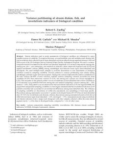
3.2. Diatom communities in relation to environmental variables Based on CCAs carried out using individual variables (Table 2), the following predictor variables were significantly (Monte Carlo permutation test, p ≤ 0.05) associated with changes in diatom communities, with a moderate to high relationship (λ 1/λ 2 N 0.5): 1) nutrient levels = TP, SRP and TN, and DO levels, 2) metal levels = Ni, Ca and Na and 3) hydromorphological factors = velocity/depth combinations, riparian vegetation zone, bank stability and percentage gravel. These variables were subsequently used in partial CCAs and the CCA conducted to explore the simultaneous effects of predictor variables from different categories. Biotic factors, i.e. macroinvertebrate grazer abundance, was not significantly associated with changes in diatom communities. From the partial CCA results, the following variations were explained by the different predictor matrices: nutrient levels and organic pollution - 10.4%, metal pollution - 8.3% and hydromorphological factors - 7.9% (Fig. 2). The results showed that 1.9% of the diatom community data variation was shared among nutrient levels and organic pollution, metal pollution and hydromorphological factors. Variation in metal pollution plus the shared variation between metal pollution and hydromorphological factors explained 11.3% - slightly higher than nutrient levels and organic pollution combined. Variation in hydromorphological factors plus the shared variation between hydromorphological factors and metal pollution explained 10.9% - slightly higher than nutrient levels and organic pollution combined. These findings from partial CCAs were strengthened by the visual CCA conducted to explore the simultaneous effects of all the predictor variables on diatom communities, where high nutrient, organically

polluted urban sampling stations were clearly separated from the rest of the sampling stations in the bottom left hand quadrant while mining sampling stations tended to be confined to the bottom right hand quadrant of the CCA (Fig. 3). These findings thus indicate clear spatial variation in diatom community structure, which is related to differences in land-use induced nutrient enrichment and organic pollution, metal pollution as well as hydromorphological alterations. The CCA clearly separated highly polluted urban sampling stations that were associated with


1609

Aulacoseira ambigua Grunow, Gyrosigma accuminatum (Kützing) Rabenhorst, and Gomphonema gracile Ehrenberg sensustricto. Agricultural sampling stations with high riparian vegetation cover were associated with species such as Aulacoseira granulata (Ehrenberg) Simonsen, Achnanthes saxonica Krasske ex Hustedt, Epithemia sorex (Kützing), Surirella ovalis Brēbisson, Fragilaria elliptica Schumann, Cymbella tumida (Brébisson) Van Heurckand Gomphonema minutum Agardh. 4. Discussion 4.1. Diatom communities in relation to environmental variables

Fig. 2. Venn diagram showing the fraction of variation explained by nutrient levels and organic pollution, metal pollution and hydromorphological predictors according to variation partitioning of diatom communities.

high SRP, TN and Ca2+ and low DO, Ni and riparian vegetation cover among other factors from the rest of the sites. Diatom species associated with these sites included pollution tolerant taxa such as Melosira varians Agardh, Frustulia vulgaris (Thwaites) De Toni, Nitzschia amphibia Grunow, Navicula seminulum Grunow, Nitzschia palea (Kützing) Smith, Gomphonema insigne Gregory and Gomphonema parvulum (Kützing) Kützing. The rest of the species, mostly of the genus Cymbella, Cocconeis, Encyonema, Eunotia, Aulacoseira, Surirella and Pinnularia, that are characteristic of moderately and less polluted environments, were associated with the other sites. Mining sampling stations were generally associated with high Na+ and Ni and DO levels and low percentage riparian vegetation among other factors. Species characterising these sites included pollution sensitive taxa species such as Navicula pupula Kützing, Pinnularia crucifera Cleve-Euler, Pinnularia divergens Smith,

Fig. 3. Canonical correspondence analysis (CCA) diagram showing simultaneous effects of nutrient levels and organic pollution, biotic factors, metal pollution and hydromorphological factors on most frequently occurring diatom taxa in the ordination space of the 1st and 2nd axes. Different symbols represent different land use patterns with circles = urban sampling stations, down triangle = mining sampling stations and crosshatch = agricultural sampling stations. Taxa codes correspond to those in Table 3.

Land-use-induced spatial variation in the levels of nutrients, organic and metal pollution and hydromorphological alterations observed in the study tropical streams have been reported in other studies (Kibena et al., 2014; Bere and Tundisi, 2011b; Nielsen et al., 2012; Tuck et al., 2014). Diatom community structure closely followed these spatial variations, with grouping of sites by CCA (Fig. 3) generally reflecting a change in community composition from highly polluted urban sampling stations to less polluted agricultural sampling stations corroborating our first hypothesis. Different diatom species in a community respond differently to nutrient enrichment, organic and metal pollution and hydromorphological alterations because of differences in tolerances developed over time. Therefore, the composition of diatom communities at different locations provides useful information about the environmental conditions. Along the agricultural b mining b urban area pollution gradient observed in this study, pollution sensitive species such as A. granulata, A. saxonica, C. tumida, E. sorex, G. minutum, G. angustatum, F. elliptica and S. ovalis were replaced by high pollution tolerant species such as M. varians, F. vulgaris, N. amphibia, N. seminulum, N. palea, G. insigne and G. parvulum which are known to be resistant to organic pollution and high ionic strength and conductivity (van Dam et al., 1994; Biggs and Kilroy, 2000). These species have also been frequently recorded in nutrient rich, poorly oxygenated, metal contaminated waters (Pan et al., 1996; Patrick and Hendrickson, 1993; van Dam et al., 1994; Biggs and Kilroy, 2000; Potapova and Charles, 2002; Bere and Tundisi, 2009; Morin et al., 2008). Ca2+ levels also played an important role in structuring benthic diatom communities in this study. Patrick and Reimer (1966) pointed out the great difference between diatom communities in calcareous and calcium-poor rivers (Fig. 2). Calcium affects diatom motility and adhesion to surfaces (Cohn and Disparti, 1994), but exact physiological mechanisms responsible for the higher or lower affinity of diatoms to calcium are still not known. Besides nutrient enrichment, organic and metal pollution, some hydromorphological factors also played an important role in structuring diatom communities in the study area. For instance, stream velocity/ depth combination was also found to be important in structuring diatom communities in the study area. High velocity sites were associated with such species as A. granulata, A. saxonica, C. tumida, E. sorex, G. minutum, G. angustatum, F. elliptica and S. ovalis. The importance of velocity in structuring benthic diatom communities has also been reported by other researchers (e.g. Patrick and Hendrickson, 1993; Biggs and Kilroy, 2000; Potapova and Charles, 2002). In addition, bank vegetation protection was also found to be important in structuring benthic diatom communities in the study area. This is because of the importance of light for diatom photosynthesis (Patrick and Hendrickson, 1993; Pan et al., 1996; Biggs and Kilroy, 2000; Potapova and Charles, 2002). Diatom communities in forested agricultural sites were, thus, different from those of open urban sampling stations. 4.2. Variation partitioning of diatom species data matrices Using partial CCA, we quantified the amount of variation in diatom species data matrices explained by different categories of environmental variables. Although observational studies like ours limit

1610


the assessment of mechanism, the amount of variation explained by nutrient enrichment, organic pollution, metal pollution and hydromorphological alterations provide us with some insight into what factors determine diatom community structure and composition in tropical streams. The inclusion of biotic factors in this study was particularly relevant since it helped to improve our understanding of the potential role of biological interactions in tropical streams for which our knowledge is still limited (Thompson et al., 2012). However, the relationship between macroinvertebrate grazer abundance and diatom community composition was insignificant. This corroborates observations by Göthe et al. (2013) where only a marginally significant relationship was observed. The variance explained by environmental factors (nutrient levels, organic and metal pollution and hydromorphological factors) dominated over biological fractions (macroinvertebrate grazer abundance). This result is supported by the notion that stream ecosystems and their communities are under strong abiotic control (Vannote et al., 1980; Göthe et al., 2013). As we hypothesised in our second hypothesis, metal levels and hydromorphological alteration explained a significant amount of variation in diatom taxonomic composition. Our partial CCA results showed that the traditional targets of current diatom-based water quality predictive models (combined nutrient levels and organic pollution) explained 10.4% of the variation in diatom communities - a value slightly higher than that attributed to metal pollution (8.3%) and hydromorphological factors (7.9%; Fig. 2). Thus, metal pollution and hydromorphological factors explained unique and significant proportions of diatom taxonomic composition in these tropical streams. In addition, variation in metal pollution plus the shared variation between metal pollution and hydromorphological factors explained 11.3% - slightly higher than nutrient levels and organic pollution combined. Variation in hydromorphological factors plus the shared variation between hydromorphological factors and metal pollution explained 10.9% - also slightly higher than nutrient levels and organic pollution combined. Since multiple stressor occurrence can be considered the rule rather than exception (Lange et al., 2011; Wagenhoff et al., 2011, 2013; Magbanua et al., 2013; Piggott et al., 2015), diatom based water quality assessment in tropical streams requires the simultaneous quantification of variation in diatom taxonomic composition across multiple stressor gradients to improve the predictive capacity of inference models. The compromise has the potential to become more useful for ‘pristine’ streams where nutrient enrichment and organic pollution have been historically low. Indeed studies in relatively pristine waters of the Eastern Highlands of Zimbabwe have shown poor applicability of some

eutrophication and organic pollution based diatom indices to assess water quality in these areas (Bere, 2015a). To our knowledge, no studies have incorporated metal pollution and hydromorphological alterations (that have been demonstrated to be important in structuring benthic diatom communities in this study) in calculation of diatom based water quality assessment predictive matrices in tropical streams, despite a plethora of different diatom-based predictive models routinely developed for inference of water quality (e.g Watanabe et al., 1986; Descy and Coste, 1991; Kelly and Whitton, 1995; Prygiel et al., 1996; Gómez and Licursi, 2001) most of which are from the temperate regions. Thus, in instances where eutrophication and organic pollution are not a major problem, current diatom-based water quality predictive models, which ignore the influence of metal pollution and hydromorphological alterations on diatom communities, are likely to give erroneous interpretations of stream water quality problems and, hence, erroneous management priorities and failing rehabilitation efforts.

5. Conclusion Our results demonstrated that factors other than nutrient levels and organic pollution, such as metal pollution and hydromorphological alterations, explain additional significant variation in diatom communities. The exclusion of these variables in development of diatom-based water quality inference models is likely to lead to erroneous inferences, especially in non-urban areas. Although the validation of these findings with experimental manipulations will be essential, the current information should encourage the development of diatom-based stream water quality inference models that incorporate metal pollution and hydromorphological alterations, resources (time and money) permitting, in tropical streams. Future attempts at precise inference of water quality in anthropogenically disturbed streams based on diatoms would require complex models incorporating information on diatom community response to metal pollution, hydromorphological alterations as well as other emerging threats such as climate change. Addressing such problems will require collaborative efforts of experts across multiple disciplines.

Acknowledgements This study was made possible by the provision of funds from British Ecological Society (BES; grant number 4218-5112) and International Foundation for Science (IFS; grant number W4848-2).


Appendix A. Habitat assessment field data sheet—high gradient streams

1611

1612



References Anderson, J.R., Hardy, E.E., Roach, J.T., Witmer, R.E., 1976. A Land Use and Land Cover Classification System For Use With Remote Sensor Data. Geological Survey Professional Paper No. 964. U.S. Government Printing Office, Washington, DC, p. 28. APHA, 1988. Standard Methods for the Examination of Water and Waste Water. 20th ed. American Public Health association, Washington, D. Barbour, M.T., Gerritsen, J., Snyder, B.D., Stribling, J.B., 1998. Rapid bioassessment protocols for use in streams and wadeable rivers: periphyton, benthic macroinvertebrates and fish. second ed. EPA/841/B/98-010 U.S. Environmental Protection Agency Office of Water, Washington, DC. Bere, T., 2015. Are diatom-based biotic indices developed in eutrophic, organically enriched waters reliable monitoring metrics in clean waters? Ecol. Indic. http://dx. doi.org/10.1016/j.ecolind.2015.11.008 (In press). Bere, T., Tundisi, J.G., 2009. Weighted average regression and calibration of conductivity and pH of benthic diatoms in streams influenced by urban pollution – Sao Carlos/ SP Brazil. Acta Limnol Brasil. 21, 317–325. Bere, T., Tundisi, J.G., 2011a. Applicability of borrowed diatom-based water quality assessment indices in streams around São Carlos-SP, Brazil. Hydrobiologia 673, 193–204. Bere, T., Tundisi, J.G., 2011b. Influence of land-use patterns on benthic diatom communities and water quality in the tropical Monjolinho hydrological basin, São Carlos-SP, Brazil. Water SA 37, 93–102. Bere, T., Mangadze, T., Mwedzi, T., 2014. The application and testing of diatom-based indices of water quality assessment in the Chinhoyi Town, Zimbabwe. Water SA 40, 503–512. Biggs, B.J.F., Kilroy, C., 2000. Stream Periphyton Monitoring Manual. NIWA, Christchurch, New Zealand. Borcard, D., Legendre, P., Drapeau, P., 1992. Partialling out the spatial component of ecological variation. Ecology 73, 1045–1055. Cohn, S.A., Disparti, N.C., 1994. Environmental factors influencing diatom cell motility. J. Phycol. 30, 818–828. Descy, J.P., Coste, M., 1991. A test of methods for assessing water quality based on diatoms. Verhand der Internat Ver für Limnol. 24, 2112–2116. Dickens, C., Graham, M., 2002. South African scoring system (SASS) version 5, rapid assessment method for rivers. Afr. J. Aquat. Sci. 27, 1–10. Gerber, A., Gabriel, M.J.M., 2002. Aquatic Invertebrates of South African Rivers. Field Guide. Institute of Water Quality Studies, Pretoria, South Africa. Gómez, N., Licursi, M., 2001. The Pampean diatom index (Idp) for assessment of rivers and streams in Argentina. Aquat. Ecol. 35, 173–181. Göthe, E., Angeler, D.G., Gottschalk, S., Löfgren, S., Sandin, L., 2013. The influence of environmental, biotic and spatial factors on diatom metacommunity structure in Swedish headwater streams. PLoS ONE 8, e72237. http://dx.doi.org/10.1371/journal.pone. 0072237. Grost, R.T., Hubert, W.A., Wesche, T.A., 1991. Field comparison of three devices used to sample substrate in small streams. N Amer J Fish Man. 11, 347–351. Jirka, A.M., Carter, M.J., 1975. Micro-semi-automated analysis of surface and waste waters for chemical oxygen demand. Anal. Chem. 47, 1397. Kelly, M.G., Whitton, B.A., 1995. The trophic diatom index: a new index for monitoring eutrophication in rivers. J. Appl. Phycol. 7, 433–444. Kibena, J., Nhapi, I., Gumindoga, W., 2014. Assessing the relationship between water quality parameters and changes in landuse patterns in the Upper Manyame River, Zimbabwe. Phys. Chem. Earth 67–69, 153–163. Korroleff, F., 1972. Determination of total nitrogen in natural water by means of persulphate oxidation. In: J.R, C. (Ed.), New Baitic Manual with Methods for Sampling and Analysis of Physical–Chemical and Biological Parameters. International council for exploration of the sea (ICES), Charlottenland. Lange, K., Liess, A., Piggott, J.J., Townsend, C.R., Matthaei, C.D., 2011. Light, nutrients and grazing interact to determine stream diatom community composition and functional group structure. Freshw. Biol. 56, 264–278. Lapš, J., Šmilauer, P., 2003. Multivariate Analysis of Ecological Data using CANOCO. Cambridge University Press. Magbanua, F.S., Townsend, C.R., Hageman, K.J., Lange, K., Lear, G., Lewis, G.D., et al., 2013. Understanding the combined influence of fine sediment and glyphosate herbicide on stream periphyton communities. Water Res. 47, 5110–5120. Metzeltin, D., Lange-Bertalot, H., 1998. Tropical Diatoms of South America II. Iconographia Diatomologica. 5, pp. 1–695. Metzeltin, D., Lange-Bertalot, H., 2007. Tropical Diatoms of South America II. Iconographia Diatomologica. 18, pp. 1–877. Morin, S., Duong, T.T., Dabrin, A., Coynel, A., Herlory, O., Baudrimont, M., et al., 2008. Longterm survey of heavy-metal pollution, biofilm contamination and diatom community

1613

structure in the Riou Mort watershed, South-West France. Environ. Pollut. 151, 532–542. Nielsen, A., Trolle, D., Søndergaard, M., Lauridsen, T.L., Bjerring, R., Olesen, J.F., Jeppesen, E., 2012. Watershed land-use effects on lake water quality in Denmark. Ecol. Appl. 22, 1187–1200. Pan, Y., Stevenson, R.J., Hill, B.H., Herlihy, A.T., Collins, G.B., 1996. Using diatoms as indicators of ecological conditions in lotic systems: a regional assessment. J N Amer Bethol Soc. 15, 481–495. Pappas, J.L., 1996. Stoermer EF, formulation of a method to count number of individuals' representative of number of species in algal communities. J. Phycol. 32, 693–696. Passy, S.I., 2007. Community analysis in stream biological monitoring: what must we measure and what we don't. Environ. Monit. Assess. 127, 409–417. Patrick, R., Hendrickson, J., 1993. Factors to consider in interpreting diatom changes. Nova Hedwig. Beih. 106, 361–377. Patrick, R., Reimer, C.W., 1966. The Diatoms of the United States. Academy of Natural Sciences, Philadelphia, p. 688. Piggott, J.J., Salis, R.K., Lear, G., Townsend, C.R., Matthaei, C.D., 2015. Climate warming and agricultural stressors interact to determine stream periphyton community composition. Glob. Chang. Biol. 21, 206–222. Potapova, M.G., Charles, D.F., 2002. Benthic diatoms in USA rivers: distributions along speciation and environmental gradients. J. Biogeogr. 29, 167–187. Proctor, J., Cole, M.M., 1992. The ecology of ultramafic areas in Zimbabwe. In: EA, R., Proctor, J. (Eds.), The Ecology of Areas with Serpentinized Rocks. A World View. Kluwer Academic Publishers, Netherlands. Prygiel, J., Lévéque, L., Iserentant, R., 1996. Unnouve lindice diatomiquepratique pour l'e´ valuation de La qualite´ des eaux en re'seau de surveillance. Revue dês Sciences de l'Eau. 1, 97–113. Prygiel, J., Whitton, B.A., Bukowska, J., 1999. Use of Algae for Monitoring Rivers III. Agence de L'Eau Artois-Picardie, Douai, p. 271. Stevens, J.R., Olsen, D.L., 2004. Spartially restricted surveys overtime for aquatic resources. J. Agric. Biol. Environ. Stat. 4, 415–425. Taylor, J.C., Harding, W.R., Archibald, C.G.M., 2007a. An Illustrated Guide to Some Common Diatom Species from South Africa. WRC Report No TT 282/07. Water Research Commission, Pretoria, South Africa. Taylor, C.J., Prygiel, A.V., de La Rey, P.A., Van Rensburg, S., 2007b. Can diatom-based pollution indices be used for biological monitoring in SA? A case study of the Crocodile West and Marico water management area. Hydrobiologia 592, 455–464. ter Braak, C.J.F., Prentice, I.C., 1988. A theory of gradient analysis. Adv. Ecol. Res. 18, 271–317. ter Braak, C.J.F., Verdonschot, P.F.M., 1995. Canonical correspondence analysis and related multivariate methods in aquatic ecology. Aquat. Sci. 37, 130–137. ter Braak, C.J.F., Šmilauer, P., 2012. Canoco Reference Manual and User's Guide: Software for Ordination (version 5.0) Microcomputer Power, Ithaca, New York. Thirion, C.A., Mox, E., Woest, R., 1995. Biological Monitoring of Streams and Rivers Using SASS4 – User Manual. Department of Water Affairs and Forestry Institute for Water Quality Studies, South Africa, p. 46. Thompson, R.M., Dunne, J.A., Woodward, G.U.Y., 2012. Freshwater food webs: towards a more fundamental understanding of biodiversity and community dynamics. Freshw. Biol. 57, 1329–1341. Tuck, S.L., Winqvist, C., Mota, F., Ahnstrcom, J., Turnbull, L.A., Bengtsson, J., 2014. Data from: land-use intensity and the effects of organic farming on biodiversity: a hierarchical meta-analysis. Dryad Digital Repos. http://dx.doi.org/10.5061/dryad.609t7. Van Dam, H., Mertens, A., Sinkeldam, J., 1994. A coded checklist and ecological indicator values of freshwater diatoms from the Netherlands. Aquat. Ecol. 28, 117–133. Vannote, R.L., Minshall, G.W., Cummins, K.W., Sedell, J.R., Cushing, C.E., 1980. River continuum concept. Can. J. Fish. Aquat. Sci. 37, 130–137. Wagenhoff, A., Lange, K., Townsend, C.R., Matthaei, C.D., 2013. Patterns of benthic algae and cyanobacteria along twin-stressor gradients of nutrients and fine sediment: a stream mesocosm experiment. Freshw. Biol. 58, 1849–1863. Wagenhoff, A., Townsend, C.R., Phillips, N., Matthaei, C.D., 2011. Subsidy-stress and multiple-stressor effects along gradients of deposited fine sediment and dissolved nutrients in a regional set of streams and rivers. Freshw. Biol. 56, 1916–1936. Wallace, J.B., Webster, J.R., 1996. The role of macroinvertebrates in stream ecosystem function. Annu. Rev. Entomol. 41, 115–139. Watanabe, T., Asai, K., Houki, A., 1986. Numerical estimation of organic pollution of flowing waters by using the epilithic diatom assemblage - diatom assemblage index (DIApo). Sci. Total Environ. 55, 209–218. William, M., Lewis, J., 2008. Physical and chemical features of tropical flowing waters. In: Dudgeon, D. (Ed.), Tropical Stream Ecology. Amsterdam, Academic Press-Elsevier, pp. 2–20.