Variational and Perturbative Extensions of Continuous Unitary ...

Variational and Perturbative Extensions of Continuous Unitary Transformations for Low-Dimensional Spin Systems

Dissertation zur Erlangung des Grades eines Doktors der Naturwissenschaften der Fakult¨at Physik der Technischen Universit¨at Dortmund

vorgelegt von

Nils Alexander Drescher aus Dortmund

21. November 2014

2

Dissertation in der Fakult¨at Physik

Technische Universit¨at Dortmund

Erster Gutachter: Prof. Dr. G¨otz S. Uhrig Zweiter Gutachter: Dr. Kai P. Schmidt Vorsitzender der Pr¨ ufungskommission: Prof. Dr. Dieter Suter Vertreterin der wissenschaftlichen Mitarbeiter: Dr. B¨arbel Siegmann Tag der m¨ undlichen Pr¨ ufung:

19.12.2014

3

Meinen Eltern Vera und Bernhard

Give me six hours to chop down a tree and I will spend the first four sharpening the ax. — Unknown. Often attributed to Abraham Lincoln. [Schwartz(2010)]

4

Contents 1 Motivation and overview 2 Self-similar continuous unitary transformations (sCUT) 2.1 Continuous unitary transformations (CUT) . . . . . . . . . 2.2 Generator schemes . . . . . . . . . . . . . . . . . . . . . . 2.2.1 Wegner’s generator scheme . . . . . . . . . . . . . . 2.2.2 Mielke’s generator scheme . . . . . . . . . . . . . . 2.2.3 Particle-conserving generator scheme . . . . . . . . 2.2.4 Particle-sorting generator schemes . . . . . . . . . . 2.3 Flow equation in second quantization . . . . . . . . . . . . 2.4 Self-similar truncation . . . . . . . . . . . . . . . . . . . . 2.5 Symmetries . . . . . . . . . . . . . . . . . . . . . . . . . . 2.5.1 Symmetries of the Hamiltonian . . . . . . . . . . . 2.5.2 Symmetries of the observable . . . . . . . . . . . . 2.6 Technical implementation . . . . . . . . . . . . . . . . . . 2.6.1 Data types . . . . . . . . . . . . . . . . . . . . . . . 2.6.2 Algorithms . . . . . . . . . . . . . . . . . . . . . . 2.6.3 Parallelization . . . . . . . . . . . . . . . . . . . . .

9 . . . . . . . . . . . . . . .

. . . . . . . . . . . . . . .

. . . . . . . . . . . . . . .

. . . . . . . . . . . . . . .

. . . . . . . . . . . . . . .

. . . . . . . . . . . . . . .

. . . . . . . . . . . . . . .

. . . . . . . . . . . . . . .

3 Enhanced perturbative continuous unitary transformations (epCUT) 3.1 Perturbative continuous unitary transformations (pCUT) . . . . . . . . . 3.2 Enhanced perturbative CUT (epCUT) for the Hamiltonian . . . . . . . . 3.2.1 Perturbative expansion of the flow equation . . . . . . . . . . . . 3.2.2 Example: Harmonic oscillator with quartic perturbation . . . . . 3.2.3 Algorithm for the Hamiltonian . . . . . . . . . . . . . . . . . . . . 3.2.4 Reduction of the differential equation system . . . . . . . . . . . . 3.3 Directly evaluated epCUT (deepCUT) . . . . . . . . . . . . . . . . . . . 3.4 Transformation of observables . . . . . . . . . . . . . . . . . . . . . . . . 3.4.1 Algorithm for the observables . . . . . . . . . . . . . . . . . . . . 3.4.2 Reduction of the differential equation system . . . . . . . . . . . . 3.5 Simplification rules for bosonic operators . . . . . . . . . . . . . . . . . . 3.5.1 Basic a posteriori rule . . . . . . . . . . . . . . . . . . . . . . . . 3.5.2 Extended a posteriori rule . . . . . . . . . . . . . . . . . . . . . . 3.5.3 Basic a priori rule . . . . . . . . . . . . . . . . . . . . . . . . . . 3.5.4 Extended a priori rule . . . . . . . . . . . . . . . . . . . . . . . . 3.6 Minimal order and symmetries . . . . . . . . . . . . . . . . . . . . . . . . 3.7 Technical aspects . . . . . . . . . . . . . . . . . . . . . . . . . . . . . . . 3.7.1 Implementation . . . . . . . . . . . . . . . . . . . . . . . . . . . .

. . . . . . . . . . . . . . .

13 14 17 17 18 18 19 20 22 25 26 28 29 31 33 37

. . . . . . . . . . . . . . . . . .

41 43 45 45 46 49 51 52 55 55 56 57 59 60 63 64 65 66 66

6

CONTENTS 3.7.2 Performance 3.8 Conclusions . . . . 3.9 Applications . . . . 3.10 Outlook . . . . . .

. . . .

. . . .

. . . .

. . . .

. . . .

. . . .

. . . .

. . . .

. . . .

. . . .

. . . .

. . . .

. . . .

. . . .

4 Variational generators 4.1 Two boson model . . . . . . . . . . . . . . . 4.2 Treatment by deepCUT . . . . . . . . . . . 4.3 Results for particle-sorting generators . . . . 4.4 Variational generators . . . . . . . . . . . . 4.4.1 Scalar optimization . . . . . . . . . . 4.4.2 Vectorial optimization . . . . . . . . 4.4.3 Tensorial optimization . . . . . . . . 4.5 Results for variational generators . . . . . . 4.5.1 Asymptotics for small off-diagonality 4.5.2 Performance for larger off-diagonality 4.6 Conclusions . . . . . . . . . . . . . . . . . . 4.7 Outlook . . . . . . . . . . . . . . . . . . . .

. . . . . . . . . . . . . . . .

. . . . . . . . . . . . . . . .

. . . . . . . . . . . . . . . .

. . . . . . . . . . . . . . . .

. . . . . . . . . . . . . . . .

. . . . . . . . . . . . . . . .

. . . . . . . . . . . . . . . .

. . . . . . . . . . . . . . . .

. . . . . . . . . . . . . . . .

. . . . . . . . . . . . . . . .

. . . . . . . . . . . . . . . .

. . . . . . . . . . . . . . . .

. . . . . . . . . . . . . . . .

. . . . . . . . . . . . . . . .

. . . . . . . . . . . . . . . .

. . . . . . . . . . . . . . . .

. . . .

70 72 73 74

. . . . . . . . . . . .

75 77 79 80 85 87 89 91 92 93 97 101 102

5 sCUTs with Variational Extensions for Dimerized Spin S=1/2 Models 105 5.1 Low-dimensional spin S=1/2 Heisenberg models . . . . . . . . . . . . . . . . 107 5.1.1 One-dimensional dimerized Heisenberg chain . . . . . . . . . . . . . 107 5.1.2 Two-dimensional dimerized Heisenberg model . . . . . . . . . . . . 108 5.2 Derivation of the effective Hamiltonian . . . . . . . . . . . . . . . . . . . . 109 5.2.1 Triplon representation . . . . . . . . . . . . . . . . . . . . . . . . . 110 5.2.2 Variational starting point . . . . . . . . . . . . . . . . . . . . . . . 111 5.2.3 Details of the CUT . . . . . . . . . . . . . . . . . . . . . . . . . . . 113 5.2.4 Symmetries . . . . . . . . . . . . . . . . . . . . . . . . . . . . . . . 114 5.3 Review: Dimerized spin S=1/2 Heisenberg chain . . . . . . . . . . . . . . . 115 5.4 Two-dimensional Heisenberg model with default starting point . . . . . . . 117 5.5 Two-dimensional Heisenberg model with varied starting point . . . . . . . 120 5.5.1 Ground state energy . . . . . . . . . . . . . . . . . . . . . . . . . . 120 5.5.2 Dispersion and gap . . . . . . . . . . . . . . . . . . . . . . . . . . . 123 5.5.3 Magnetization . . . . . . . . . . . . . . . . . . . . . . . . . . . . . . 127 5.6 One-dimensional Heisenberg chain with generic optimization of starting point128 5.6.1 Stepwise optimization of starting point . . . . . . . . . . . . . . . . 129 5.6.2 Continuous optimization of starting point . . . . . . . . . . . . . . 130 5.7 Conclusions . . . . . . . . . . . . . . . . . . . . . . . . . . . . . . . . . . . 133 5.8 Outlook . . . . . . . . . . . . . . . . . . . . . . . . . . . . . . . . . . . . . 135 6 S=1 Heisenberg chain by deepCUTs 6.1 S=1 Heisenberg chain . . . . . . . . . . . . . . . . . . . 6.2 Treatment by deepCUT with variational extensions . . 6.2.1 Mapping to S=1/2 Heisenberg ladder . . . . . . 6.2.2 Triplon Hamiltonian and observables . . . . . . 6.2.3 Decoupling of the low quasi-particle sub-spaces 6.2.4 Evaluation of spectral properties . . . . . . . . 6.3 Selection of the variational parameter . . . . . . . . . . 6.4 Overview over the energy spectrum . . . . . . . . . . .

. . . . . . . .

. . . . . . . .

. . . . . . . .

. . . . . . . .

. . . . . . . .

. . . . . . . .

. . . . . . . .

. . . . . . . .

. . . . . . . .

. . . . . . . .

137 . 138 . 139 . 139 . 141 . 143 . 145 . 148 . 151

CONTENTS 6.5 6.6 6.7 6.8

Details of the S=0 spectrum Details of the S=1 spectrum Conclusions . . . . . . . . . Outlook . . . . . . . . . . .

7 . . . .

. . . .

. . . .

. . . .

. . . .

. . . .

. . . .

. . . .

. . . .

. . . .

. . . .

. . . .

. . . .

. . . .

. . . .

. . . .

. . . .

. . . .

. . . .

. . . .

. . . .

. . . .

. . . .

. . . .

. . . .

. . . .

153 159 164 165

7 Summary

167

8 Zusammenfassung

169

A Dispersions of the Two-dimensional Dimerized S=1/2 Heisenberg Model171 Bibliography

187

Teilpublikationen

189

Danksagung

191

8

CONTENTS

Chapter 1 Motivation and overview Superconductivity is one of the most impressing quantum phenomena that can be observed macroscopically. Since its discovery by Onnes [Onnes(1911), Onnes(1913)], the exotic properties of the superconducting phase have triggered numerous theoretical and experimental studies, and as well as extensive research for industrial applications [Bray(2008), Bray(2009)]. Apparently, the ability of superconducting materials below their transition temperature Tc to carry high current densities without any losses due to electrical DC resistance is attractive in numerous technological applications. First of all, we mention the generation and indefinite maintenance of strong magnetic fields used in research facilities, particle accelerators like the Large Hadron Collider (LHC), and for compact and lightweight electric motors and generators. So far, the biggest commercial success has been achieved by superconducting solenoids for Magnetic Resonance Imaging (MRI) devices, which provide an exceptionally high resolution for medical diagnostics without the ohmic losses and heat production of conventional copper solenoids. An obvious application of superconductivity are superconducting wires for connecting of electrical power grids. However, superconductors are also suitable for the construction of more sophisticated power grid components, e. g. fault current limiters or superconducting magnetic energy storage. Moreover, superconductors can be used in an increasing number of electronic devices, with high quality microwave filters in cell phone base stations being the most successful commercial application [Smith & Jain(1999),Willemsen(2001)]. The exploitation of the Josephson effect in superconducting quantum interference devices (SQUIDs) allows for the measurement of magnetic fields with the accuracy of flux quanta. Eventually, the direct manipulation of magnetic flux quanta in superconducting quantum circuits is a promising candidate for the implementation of scalable quantum computers [Barends et al.(2014)]. Microscopically, the superconducting phase can be understood as condensate of twoelectron bound states (Cooper pairs). For conventional superconductivity, as it has been found in pure metals or alloys like NbTi, the attractive interaction between electrons is mediated by electron-phonon coupling [Bardeen et al.(1957b),Bardeen et al.(1957a)]. The need to operate well below the transition temperature of the superconductor diminishes the technical and economical benefits of superconducting devices, since the low transition temperatures of conventional superconductors require expensive cooling by liquid helium. For this reason, much interest has been paid to the discovery of unconventional superconductors [Bednorz & M¨ uller(1986)], where the conventional, phonon-mediated mechanism can be ruled out due to the missing isotope effect [Hoen et al.(1989)]. While

10

Motivation and overview

different classes of unconventional superconductors have been found over the years, the pairing mechanism in this materials remains one of the most puzzling open questions in condensed matter physics. Of particular interest are cuprate superconductors, some of which remain superconducting above the boiling point of liquid nitrogen [Wu et al.(1987)] and even up to 138 K [Dai et al.(1995)], leading to the name high-temperature superconductor (HTSC). While their high transition temperature makes them more attractive than conventional superconductors for industrial applications, the manufacturing process is more challenging. The understanding of the pairing mechanism in HTSCs is of great interest for fundamental research. At the same time, it has as a strong technological motivation, as it might lead to novel superconducting materials with even higher transition temperatures and improved mechanical properties, allowing for the widespread application of superconducting technologies. Chemically, the cuprate superconductors consist of low-dimensional structures (chains, ladders, plains) of copper and oxygen, embedded in a matrix of various other elements. While the host materials like La2 CuO4 are believed to be Mott insulators [Manousakis(1991)], doping with electrons or holes leads to normal conductance by charge carriers and, at a critical concentration, superconductivity arises. Interestingly, the materials enter the superconducting state close to the breakdown of long-range anti-ferromagnetic (AFM) order, where a quantum phase transition (QPT) to a magnetically disordered ground state happens. This suggest that the attractive interaction between charge carriers in cuprate HTSCs is mediated by magnetic fluctuations, and particular interest has been paid on the magnetic properties of the ground state and its excitations. Because cuprate superconductors have a complex chemical and geometrical structure, complex interactions and strong electronic correlations to consider, a direct description taking all microscopic details into account seems to be desperate. In order to provide an understanding of the mechanisms that are essential for the magnetic properties and, finally, their role in the mechanism of superconductivity, a stepwise reduction of complexity is necessary. In the cuprates, the half-occupied orbitals of the Cu2+ ions is most important for the electronic and magnetic properties. They interact via superexchange mediated by the oxygen atoms. This system can be simplified as a Hubbard model, where each lattice site represents one orbital of a copper atom that can hold up to two electrons. In the minimal realization, only Coulomb repulsion U on the same site and a nearest-neighbour hopping t are considered as interactions. For the undoped case, i. e., for one electron per lattice site and in the limit of large U  t, the system becomes a Mott insulator, where each electron is confined to a specific site and electron hopping is inhibited by the high energy of doubly occupied states. For studying the low-energy physics of the system, it is sufficient to concentrate on the spin degree of freedom of the localized electrons. This leads us to the Heisenberg model, which describes the system in terms of effective spin-spin interactions that are a consequence of the high-energy physics in the underlying Hubbard model. At each of these steps, processes on a large energy scale determine the properties on a lower energy scale in an intricate way. This gives rise to a large variety of effective interaction processes that appear in the effective low-energy model. Depending on which effective couplings are identified as important and which can be neglected in different parameter regimes of the macroscopic model, it can be necessary to construct different effective models in order to understand the macroscopic model in all aspects. Conversely, new insights can be gained when the couplings of the effective model are treated as free

11 parameters and the full phase diagram is explored, giving rise to novel kinds of order, exotic phases and their excitations. Continuous unitary transformations (CUT) are a powerful framework to derive such effective low-energy models in a systematic and controlled fashion. By selection of an appropriate generator scheme, they offer a large degree of control over the general structure of the derived effective model. Even more, they can be used to understand the physical properties of the system in terms of conserved quasi-particles for the elementary excitations and to describe multi-particle continua and bound states, as well as response functions. The effective Hamiltonian can be diagonalized directly by the continuous unitary transformation (CUT), or used as starting point for the investigation by other methods. In this thesis, we derive several methodological improvements of the CUT method, including perturbative and variational aspects, and apply it to low-dimensional spin systems. The thesis is structured as follows: In chapter two, we give an introduction to the self-similar CUT (sCUT) method that serves as a starting point for the studies in the subsequent chapters and explain the computational implementation used in this thesis. In chapter three, we develop two novel CUT-based techniques to study many-particle systems: The enhanced perturbative CUT (epCUT) method, which allows for high-order perturbative expansions for effective models beyond the limitations the existing perturbative CUT (pCUT) approach, and the directly evaluated epCUT (deepCUT) method, which allows us to obtain non-perturbative effective Hamiltonians efficiently and with a significantly larger robustness compared to sCUT. We illustrate these methods by a perturbed harmonic oscillator as pedagogic example. In chapter four, we investigate the properties of CUTs in second quantization for systems with overlapping quasi-particle sub-spaces. These systems are a particular challenge for the CUT method, because the particle-sorting generator schemes used to decouple the low-energy spectrum can fail in the case of strong overlap or yield a misleading quasi-particle picture. We investigate this in detail for a system of two coupled harmonic oscillators using deepCUT. Then, we develop a family of three novel variational generator schemes that do not suffer from the problems of the conventional particle-sorting generators. They lead to a meaningful quasi-particle interpretation even in the case of strong overlap. In chapter five, we study the QPT in the dimerized, two-dimensional S=1/2 Heisenberg model by means of sCUT with a variational starting point. For the first time, we are able to describe a phase with a spontaneously broken continuous symmetry by means of CUT and to derive an effective model that describes both gapped triplons and gapless magnons as quasi-particles in a uniform operator representation. After this, we generalize the concept of the variational starting point and show how an optimal starting point can be obtained independent of the particularities of the model. In chapter six, we investigate the S=1 Heisenberg chain using the deepCUT method and derive an effective model in terms of triplon quasi-particles. To this end, we use a mapping to a ladder-like S=1/2 Heisenberg system introducing a variational parameter. We analyze the low-energy spectrum and calculate energy- and momentum-resolved response functions. In particular, we are interested in the spontaneous quasi-particle decay of one triplon into two triplons. We find that, due to the strongly overlapping quasi-particle sub-spaces, the use of the variational generators is mandatory. Finally, we summarize our findings in both English and German language.

12

Motivation and overview

Chapter 2 Self-similar continuous unitary transformations (sCUT) Contents 2.1

Continuous unitary transformations (CUT)

. . . . . . . . . .

14

2.2

Generator schemes . . . . . . . . . . . . . . . . . . . . . . . . . .

17

2.2.1

Wegner’s generator scheme . . . . . . . . . . . . . . . . . . . .

17

2.2.2

Mielke’s generator scheme . . . . . . . . . . . . . . . . . . . . .

18

2.2.3

Particle-conserving generator scheme . . . . . . . . . . . . . . .

18

2.2.4

Particle-sorting generator schemes . . . . . . . . . . . . . . . .

19

2.3

Flow equation in second quantization . . . . . . . . . . . . . .

20

2.4

Self-similar truncation

. . . . . . . . . . . . . . . . . . . . . . .

22

2.5

Symmetries . . . . . . . . . . . . . . . . . . . . . . . . . . . . . .

25

2.6

2.5.1

Symmetries of the Hamiltonian . . . . . . . . . . . . . . . . . .

26

2.5.2

Symmetries of the observable . . . . . . . . . . . . . . . . . . .

28

Technical implementation . . . . . . . . . . . . . . . . . . . . .

29

2.6.1

Data types . . . . . . . . . . . . . . . . . . . . . . . . . . . . .

31

2.6.2

Algorithms . . . . . . . . . . . . . . . . . . . . . . . . . . . . .

33

2.6.3

Parallelization . . . . . . . . . . . . . . . . . . . . . . . . . . .

37

At first glance, condensed matter physics might appear as terra cognita: Schr¨odinger’s equation, the theory of everything at low energy scales, and the basic ingredients, electrons and nuclei, are known since the early 20th century; the Hamiltonian of any compound can be written down exactly [Czycholl(2000)]. De facto, the complex interactions between these comparatively simple building blocks in various geometries have proven to be a cornucopia of innumerable interesting and diversified physical phenomena. The challenges in understanding these phenomena go well beyond a mere quantitative reproduction; a significant reduction of complexity by suitable representations, smart approximations and powerful effective theories is essential. In the best case, even rough approximations can provide an understanding for the essential ingredients of complex physical phenomena. Prominent examples comprise the concepts of quasi-particles and Fermi liquid theory [Landau(1957)]. They allow for the description

14

Self-similar continuous unitary transformations (sCUT)

of a complex, strongly-interacting, highly-correlated many-fermion-system in terms of the well-known, interaction-free Fermi gas, modified by just a few material-specific parameters that can be determined experimentally. In the attempt to map a physical system to a renormalized Hamiltonian, where the phenomena of interest are better accessible, unitary transformations turned out to be a very versatile and powerful tool. They bear the advantage to retain the spectrum of eigenvalues when mapping a Hamiltonian to an effective model. In this manner, they allow us to decouple different degrees of freedom, e. g., different types of quasi-particles, or to map a many-particle problem to a few-particle problem of conserved quasi-particles. In this way, the high-energy processes can be integrated out and an effective model for the low-energy physics is obtained. Eventually, the effective model can be studied by standard techniques or the degrees of freedom on the low-energy scale can be decoupled and studied individually. Depending on the realization, different limitations appear: For a numerical, exact diagonalization to be feasible, the Hilbert space has to be kept finite, implying a finite lattice size. Some one-step transformations such as the Bogoliubov transformation [Bogoliubov(1958a), Bogoliubov(1958b)] can be applied completely on an analytical level, but they decouple any but the most simple Hamiltonians to a limited degree only. Other unitary transformations such as the Fr¨ohlich transformation [Fr¨ohlich(1952)] require additional approximations. Another technique that relies on a multi-step transformation is the projector-based renormalization method [Becker et al.(2002)]. In this thesis, we focus on an approach that can be understood as an infinite number of infinitesimal unitary transformations, leading to a continuous unitary transformation (CUT), that maps the Hamiltonian to an effective model. The structure of the effective model is controlled by the generator scheme. In this chapter, we introduce the CUT with a focus on its self-similar version. We start with a discussion of CUT and the flow equation in general. In the second section, we present the various generator schemes used to derive effective Hamiltonians of different shapes. Then, we introduce a formulation of the flow equations using second quantization. Based on this, we explain the truncation scheme characteristic for self-similar CUTs in section 2.4. In the subsequent section, we describe a formalism to exploit the symmetries of the Hamiltonian in second quantization. Finally, we illustrate the key concepts of the computational implementation used in this thesis with emphasis on parallelization.

2.1

Continuous unitary transformations (CUT)

Finding a suitable transformation to map the initial Hamiltonian Hinit to an effective Hamiltonian Heff of a specific shape is a sophisticated task. For a one-step transformation, it requires to anticipate the action of a possibly very complex transformation as a whole, while minimizing deviations from the desired structure of the effective Hamiltonian. The CUT method found independently by Wegner [Wegner(1994)] and Glazek and Wilson [Glazek & Wilson(1993), Glazek & Wilson(1994)] circumvents these problems using an infinite number of infinitesimal transformations, each of them bringing the Hamiltonian closer to the desired shape. Mathematically, this translates into the parametrization of the transformation H(`) := U (`)HU † (`)

(2.1)

2.1 Continuous unitary transformations (CUT)

15

by a continuous flow parameter ` with the initial condition U (0) = 1

⇒

H(0) = Hinitial

(2.2)

and Heff := H(∞). At each value of `, the momentary infinitesimal transformation can be understood in terms of the antihermitian generator η(`) =

∂U (`) † U (`) = −η † (`) ∂`

(2.3)

of U (`). By this definition, the flow of the Hamiltonian (2.1) can be described by a differential equation, denoted as flow equation ∂` H = [η(`), H(`)].

(2.4)

In this notation, the control of the direction of the flow has been shifted from U (`) to the generator η(`). The main advantage of this formulation is that the generator can be chosen as a function η(`) = ηb [H(`)]

(2.5)

of the flowing Hamiltonian itself, defined by a superoperator ηb that we call generator scheme henceforth. Therefore, it is not necessary to store the full, possibly very complex transformation U (`). Due to the feedback of the Hamiltonian on the generator, the flow equation (2.4) is non-linear. As a consequence, a suitable generator scheme can steer the generator asymptotically towards attractive fixed points of the flow equation where the Hamiltonian has the desired simpler structure. The variety of possible generator schemes allows for a large degree of control over the shape of the effective Hamiltonian. We give an overview of the various possibilities in the next section. For the calculation of experimentally observable quantities such as static correlations or response functions, two aspects of CUT matter: If the Hamiltonian is transformed into the renormalized basis, its structure can be chosen in a way that the determination of the ground state and excited states is easier or even trivial. However, the associated operator O has to be known in the same basis. This is achieved by the transformation of observables ∂` O = [η(`), O(`)].

(2.6)

This has been used for the first time by Kehrein and Mielke [Kehrein & Mielke(1998), Kehrein(1999)] in their studies of dissipative quantum systems. Since the generator η(`) has to be determined by the flowing Hamiltonian, it is preferable to carry out the integration of both equations (2.4) and (2.6) simultaneously. While the global structure of the Hamiltonian may become simpler in the sense that different degrees of freedom are decoupled, new interaction processes arise in the flowing Hamiltonian due to the commutator in Eq. (2.4). They have to be considered as arguments of the commutator again. In any, but the most simple situations, the ensuing proliferation of more and more interaction processes leads to an infinite number of terms and the differential equations are not closed. Different strategies have been suggested to handle this problem leading to different realizations of CUTs:

16

Self-similar continuous unitary transformations (sCUT)

Restriction to finite systems: If the system is restricted to a finite size, i. e., the Hamiltonian is a matrix of finite dimension, the flow equation can always be closed. Inevitably, this places a severe limitation on the application to systems in the thermodynamic limits. Perturbative CUT (pCUT): The idea of a perturbative expansion is continued systematically in the pCUT method by Knetter and Uhrig [Uhrig & Normand(1998),Knetter & Uhrig(2000), Knetter et al.(2003a)], which allows us to derive a perturbative expansion for the effective Hamiltonian up to very high orders. Under the requirements of pCUT, the perturbative flow equations can be integrated analytically and the remaining task consists in the calculation of matrix elements of the effective Hamiltonian. We will give a short overview of this method in section 3.1. Self-similar CUT (sCUT): This version of CUT is the focus of this chapter. The Hamiltonian is approximated by a large but finite number of interaction processes in second quantization. The systematics which processes are considered is defined in the truncation scheme, cf. Sect. 2.4, based on a small parameter [Mielke(1997b), Mielke(1997a), Kehrein(2006)] or with respect to the range of the underlying process in real-space [Reischl et al.(2004), Fischer et al.(2010), Duffe(2010)]. For these processes, the flow equation is integrated numerically, giving rise to a non-perturbative, renormalized Hamiltonian. Graph-theory based CUT (gCUT): In the gCUT method [Yang & Schmidt(2011)] developed recently, the action of the Hamiltonian is decomposed into the action on finite graphs of various complexity. On each graph, the flow equation for the Hamiltonian can be solved numerically on the matrix level. At the end, the irreducible contributions of each graph are combined to obtain a non-perturbative effective Hamiltonian valid in the thermodynamic limit. This method can be seen as an extension of the exact linked-cluster expansion [Irving & Hamer(1984)] for ground-state properties. The accuracy is controlled by the maximal size of the graphs, similar to the range of processes in a sCUT with real-space truncation. Enhanced perturbative CUT (epCUT): The epCUT method combines elements of both pCUT, i. e., the perturbative expansion of Hamiltonian and flow equation, and sCUT, i. e., the representation of the Hamiltonian in second quantization and the explicit numerical integration of the resulting differential equation system (DES) for its coefficients. By this combination, it is possible to overcome the limitations of pCUT and obtain effective Hamiltonians for a larger class of models. In addition, the special truncation of the flow equations associated with epCUT gives rise to a non-perturbative twin, the directly evaluated epCUT (deepCUT) method. The epCUT and the deepCUT have been developed by Holger Krull [Krull(2011),Krull et al.(2012)], G¨otz Uhrig and myself; my contribution is expounded in chapter 3 of this thesis. Due to their high flexibility, CUT-based methods have been applied to a large range of models. For an overview of the different applications, we recommend references [Kehrein(2006), Wegner(2006)] and [Krull et al.(2012)].

2.2 Generator schemes

2.2

17

Generator schemes

The choice of the generator scheme implies a large degree of control over the mapping of the initial Hamiltonian to the effective model in the limit of infinite `. A qualitative understanding of the flow induced by a generator scheme is provided by the fixed points of the flow. If the flowing Hamiltonian converges in the limit of infinite `, the effective Hamiltonian has to commute with the generator `→∞

[η(`), H(`)] −→ 0

(2.7)

and the flow equation approaches a fixed point. Since the generator is determined from the Hamiltonian itself, the generator scheme puts a necessary condition on the effective Hamiltonian’s structure, e. g. diagonality or block-diagonality. In a second step, the asymptotics of the flowing Hamiltonian in the vicinity of the fixed points can be studied. The flowing Hamiltonian can converge only to attractive fixed points, unless the initial Hamiltonian corresponds to a stationary point already1 . However, the existence of attractive fixed points alone does not guarantee that the flowing Hamiltonian converges. The set of Hamiltonians for which the generator scheme converges is a third criterion that can be used to classify different generator schemes.

2.2.1

Wegner’s generator scheme

At first, we consider the original generator scheme introduced by Wegner [Wegner(1994)]. For each value of the flow parameter, the Hamiltonian H(`) = Hd (`) + Hnd (`) is decomposed into a diagonal part Hd (`) and an off-diagonal part Hnd (`) that shall vanish for infinite `. Taken literally, this means to include any matrix element between different states in Hnd . However, we are completely free to include only a part of these matrix elements in Hnd ; the rest is assigned to Hd (`) and converges to a finite value for ` → ∞. For this reason, the term “diagonal” is often used sloppily in the context of generator schemes and denotes the parts of the Hamiltonian to be kept. For a many-particle problem for instance, it is meaningful to decouple subspaces of different quasi-particle number leading to a block-diagonal effective Hamiltonian [Wegner(1994)]. With this decomposition, Wegner’s generator is defined as ηW (`) = ηbW [H(`)] = [H(`), Hnd (`)] = [Hd (`), Hnd (`)].

(2.8a)

On the matrix level, the generator can be written as ηW,ij (`) = (hii (`) − hjj (`))hij (`).

(2.8b)

The generator depends bilinear on the Hamiltonian’s coefficients, which yields a trilinear flow equation. Because the squared Frobenius norm of the diagonal part X X ||Hd (`)||2 = |hii (`)|2 = 2 (hii (`) − hjj (`))2 hij (`)hji (`) (2.9) i

1

ij

If the Hamiltonian has a special symmetry, a third case is possible in which the Hamiltonian converges to a saddle point protected by symmetry.

18

Self-similar continuous unitary transformations (sCUT)

is increasing monotonically and bounded from above, the flowing Hamiltonian has to converge always to a fixed point, where all off-diagonal elements hij vanish or connect degenerate states with hii = hjj . The original proof for finite matrices [Wegner(1994)] has been extended to infinite systems [Dusuel & Uhrig(2004)] and self-similar truncation [Moussa(2010)], the latter one including a derivation of the generator scheme based on a variational argument.

2.2.2

Mielke’s generator scheme

In 1998, Mielke proposed a different generator [Mielke(1998)] defined on the matrix level that depends explicitly on the row and column indices ηM,ij (`) = sign(i − j)hij (`).

(2.10)

In contrast to Wegner’s generator, it vanishes only if all matrix elements between different states are zero, even in presence of degeneracies. The flow equations for the matrix elements of the Hamiltonian read ∂` hij (`) = − sign(i − j) (hii (`) − hjj (`)) hij (`) X (sign(i − k) + sign(j − k)) hik (`)hkj (`). +

(2.11)

k6=i,j

In the vicinity of fixed points of the flow, i. e., diagonal Hamiltonians, the derivative is dominated by the leading term linear in the off-diagonality. A fixed point is attractive if sign(i − j) = sign(hii (∞) − hjj (∞))

(2.12)

holds, which means that the eigenvalues have to be sorted in ascending order in the energy at ` = ∞ if the corresponding states have been linked by matrix elements in the course of the flow. Another interesting feature of this generator scheme appears if the initial Hamiltonian exhibits a band-diagonal structure, i. e., for a fixed N ∈ N holds hij = 0 if |i − j| > N . In this case, the sign functions in Eq. (2.11) ensure that the differentials of off-diagonal elements violating the band-diagonality never become finite [Mielke(1998)]. Eventually, this conservation of the band-diagonality limits the emergence of higher interaction terms, which improves the numerical performance. The convergence of this generator scheme can be proven by investigation of the sum of the first r diagonal elements of H, which turns out to be a monotonically decreasing function of `. If the spectrum of H is bounded from below, the sum has to converge while the off-diagonal elements connecting the first r states to higher states vanish [Mielke(1998)]. This proof holds for both finite and infinite matrices. However, the norm of the offdiagonality itself can increase in early phases of the flow due to the sorting of eigenvalues enforced by Eq. (2.12) [Dusuel & Uhrig(2004)].

2.2.3

Particle-conserving generator scheme

A related generator scheme has been suggested by Knetter and Uhrig [Uhrig & Normand(1998), Knetter & Uhrig(2000), Knetter(1999)] for the purpose of decoupling subspaces with different quasi-particle numbers ηpc ij (`) = sign (qii − qjj ) hij (`).

(2.13a)

2.2 Generator schemes

19

This scheme can be seen as a generalization of Mielke’s generator scheme where the indices i and j are replaced by the diagonal elements qii and qjj of an operator Q that is already in its eigen basis [Knetter et al.(2003b)]. In this way, each state i has a well-defined quantum number qii and the generator acts only between states of different qii . We emphasize that the operator Q is not transformed as an observable, so that the labeling by qii is permanent, whereas the commutator [H(`), Q] changes during the flow. For the decoupling of subspaces with different quasi-particle numbers in many-body problems, Q can be identified with the quasi-particle counting operator. This leads to the name “particle-conserving generator scheme”, because the number of renormalized quasi-particles at ` = ∞ is a conserved quantum number. In this context, the subspace of zero quasi-particle can be a unique reference state, i. e., the vacuum of quasi-particles, or a reference ensemble that can have other quasi-particles as degrees of freedom, giving rise to the systematic derivation of effective low-energy models. The definition (2.13a) can be expressed also in second quantization as ηbpc [H(`)] =

X i>j

Hji (`) − Hij (`),

(2.13b)

where Hji stands for the block of the Hamiltonian that creates i and annihilates j quasiparticles. This representation is especially useful for the application in the thermodynamic limit. As for Mielke’s generator scheme, convergence can be guaranteed if the spectrum is bounded from below [Knetter & Uhrig(2000)]. If approximations are used however, the flow equations can diverge even in this situation [Dusuel & Uhrig(2004), Reischl(2006)]. If the ground state is unique, the particle-conserving generator scheme maps vacuum state of the renormalized basis to the physical ground state of the system [Heidbrink & Uhrig(2002)]. This proof has been generalized in the sense that the particle-conserving generator sorts all quasi-particle subspaces in such a way that all energy eigenvalues are ascending by their quasi-particle number [Fischer et al.(2010)]. In analogy to Mielke’s generator scheme, ηbpc conserves the block-band diagonal structure of the initial Hamiltonian, i. e., a Hamiltonian composed of terms that change the quasi-particle number by at most ∆QP keeps this property in the course of the flow [Knetter & Uhrig(2000), Knetter et al.(2003b)]. A similar generator scheme has been used previously by Stein at al. for the Hubbard model [Stein(1997)] and Holstein-Primakov bosons [Stein(1998)], where the sign function was not necessary to conserve the block-band diagonal structure of the Hamiltonian because changes of the boson number occurred only by a fixed number, namely ±2.

2.2.4

Particle-sorting generator schemes

The particle-conserving generator scheme allows us to decouple and to sort all quasi-particle subspaces ascending by energy. This full sorting can be problematic if physics of the model suggests an effective model with overlapping quasi-particle subspaces. In these situations, the particle-conserving generator scheme rearranges the Hilbert space in an inappropriate way and causes the flow equations to diverge in presence of approximations [Reischl(2006), Fischer et al.(2010)]. To overcome these problems, Fischer, Duffe and Uhrig introduced a family of generator

20

Self-similar continuous unitary transformations (sCUT)

schemes ηbm:n [H(`)] =

XX j≤m i>j

Hji (`) − Hij (`)

(2.14)

that only decouple and sort the m lowest quasi-particle subspaces, while higher subspaces remain coupled [Fischer(2007), Duffe(2010), Fischer et al.(2010), Duffe & Uhrig(2011), Fischer(2012a)]. In the following, we refer to them as ’particle-sorting generator schemes’, with ηbpc as a special case. This approach also bears the advantage that fewer commutators have to be calculated, even though the block-band diagonality can no longer be guaranteed. We develop this concept further in chapter 4. One of the first applications of the particle sorting generator schemes has been the successful description of spontaneous quasi-particle decay in the S = 1/2 Heisenberg chain with diagonal coupling [Fischer et al.(2010), Fischer(2012a)], where the dispersion enters and hybridizes with the two-quasi-particle continuum. The ground-state generator η0:n is used to decouple the ground state only, while the remaining interactions between the one-particle dispersions and higher subspaces are treated by a variational diagonalization in a finite subspace. A similar strategy has been applied recently to calculate the low-energy excitations of the ionic Hubbard model [Hafez et al.(2014a), Hafez et al.(2014b)]. In 2008, Dawson et al. independently derived a similar generator ηDEO,ij (`) = hi,0 (`)δ0,j − δi,0 h0,j (`)

(2.15)

that takes into account only matrix elements between vacuum and higher states [Dawson et al.(2008)]. We stress that, in contrast to the particle-conserving generator scheme, the definition on the matrix level versus second quantization is not just a matter of notation, but actually leads to different flows since η0:n , for instance, comprises also matrix elements between the one quasi-particle sector and higher subspaces, in contrast to ηDEO . Interestingly, the flow of the vacuum energy E(`) = h0| H(`) |0i for the generators ηpc , η0:n and ηDEO turns out to be identical for a unique vacuum state and without approximations [Fischer et al.(2010), Fischer(2012a)].

2.3

Flow equation in second quantization

In its standard formulation (2.4), the flow equation is a differential equation for the Hamiltonian as an operator which is a complicated object that is beyond the scope of standard integration algorithms. Apart from the treatment on the matrix level, the formulation of CUT in second quantization [Wegner(1994),Dusuel & Uhrig(2004),Reischl et al.(2004), Knetter et al.(2003a), Fischer et al.(2010)] allows us to extract an ordinary DES for scalar, `-dependent functions hi (`) as prefactors of terms in the Hamiltonian2 . To this end, we define an operator basis {Ai }, consisting of normal-ordered monomials of creation and annihilation operators together with the identity operator. The name “term” is reserved for the combination of a monomial and its scalar prefactor. Using these definitions, we expand the Hamiltonian X H(`) = hi (`)Ai . (2.16) i 2

c This section is based on my contribution to the article [Krull et al.(2012)]. 2012 American Physical Society.

2.3 Flow equation in second quantization

21

using the basis {Ai } and the `-dependent coefficients hi (`). In the following, we restrict ourselves to the particle-sorting generator schemes because the application of these generator schemes to a term corresponds to a multiplication with a sign factor ci ∈ {−1, 0, +1}. Then, the generator can be written as X X η(`) = ηi (`)Ai := hi (`)ˆ η [Ai ]. (2.17) i

i

Expanded in the operator basis, the flow equation (2.4) reads X X ∂` hi (`)Ai = hj (`)hk (`) [b η [Aj ], Ak ] . i

(2.18)

jk

Comparing the coefficients of different monomials, the flow equation (2.4) finally becomes equivalent to a set of ordinary differential equations for the coefficients hi (`) X ∂` hi (`) = Dijk hj (`)hk (`). (2.19a) jk

The commutator relations between the basis operators are encoded in the coefficients Dijk of the bilinear DES. These coefficients Dijk are complex numbers in general . For the systems considered in this thesis they are given by integers or fractional numbers. We call a single Dijk a “contribution” to the DES. The contributions are obtained from X [b η [Aj ], Ak ] = Dijk Ai (2.19b) i

by comparing the coefficients of the result of the commutator monomial by monomial. In this way, the problem of solving the flow equation is transformed into the algebraic problem of calculating the coefficients of the DES (2.19b) and of the subsequent numerical solution of Eq. (2.19a). To assess the level of convergence realized by the particle-sorting generators during the integration, it is advantageous to measure the residual off-diagonality (ROD) of the Hamiltonian in the sense of terms that have to be rotated away by the generator. In this thesis, we use the Pythagorean sum of the Hamiltonian’s coefficients of all terms that contribute to the generator s X 2 |ηi | , (2.20) ROD = i

that differs from Reischl’s original definition [Reischl et al.(2004), Reischl(2006)] by a square root. For lattice systems, it is necassary to consider the coefficients of terms related by translation invariance in the sum only once in order to guarantee a finite ROD. The formulation in second quantization can be extended straightforwardly to observables X O(`) = oi (`)Bi (2.21) i

with coefficients oi (`), while the corresponding operator basis Bi does not need to be the same as for the Hamiltonian. Hence the flow equation for an observable (2.6) leads to a DES for its coefficients X obs ∂` oi (`) = Dijk hj (`)ok (`). (2.22a) j,k

Self-similar continuous unitary transformations (sCUT)

H

η

∂ℓ

η

O

O

H

∂ℓ

22

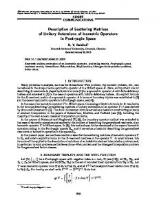
Figure 2.1: Schematic representation of the sCUT self-consistency loops. The sets of monomials are represented by the sides of the rectangle, while each area represents the set of commutators between pairs of monomials. The inner lines separate the different iterations of the sCUT algorithm. Left panel: Self-consistency loops for the Hamiltonian. Usually, both H and η refer to the same operator basis. Right panel: Self-consistency loops for an observable.

obs The contributions Dikj are obtained by calculating the commutators between the monomials of the generator and the monomials of the observable followed by a comparison of the coefficients X obs Dijk Bi = [ˆ η [Aj ], Bk ] . (2.22b) i

The DES for the coefficients of the observables is linear, but it is coupled to the transformation of the Hamiltonian via the prefactors hj (`).

2.4

Self-similar truncation

The characteristic approximation of the sCUT method consists in restricting the flowing Hamiltonian to a finite set of basis operators {Ai }, denoted as truncation scheme. By this, the flowing Hamiltonian is confined to a finite-dimensional sub-manifold of the operator algebra. All commutators between the relevant {Ai } are taken into account to determine the DES. Technically, this is done by calculating all the commutators for monomials present in the initial Hamiltonian first. If further monomials compatible with the truncation scheme arise in the calculation, they are added to the set of basis operators and the missing commutators are calculated. This step is iterated until no new basis operators incorporated by the truncation scheme arise [Reischl(2006), Duffe(2010)]. A schematic representation is given in Fig. 2.1. The sCUT strategy is optimal in the sense that the truncated flow is chosen as close to the untruncated flow-line as possible without violating the truncation criterion, i. e., the Frobenius/Hilbert-Schmidt norm of the neglected part of the flowing Hamiltonian is minimal for each value of ` [Moussa(2010)].

2.4 Self-similar truncation

α

α

β

β

γ

γ |αβγihαβγ|

23

α

αα

αα

αα

α

β

ββ

ββ

ββ

β

γ

γ γ

1

γ γ

γ γ a†β aβ

a†α aα

γ a†γ aγ

α

αα

αα

αα

α

β

ββ

ββ

ββ

β

γ

γ γ a†α a†β aα aβ

γ γ a†β a†γ aβ aγ

γ γ a†α a†γ aα aγ

γ a†α a†β a†γ aα aβ aγ

Figure 2.2: Decomposition of the diagonal matrix element |αβγi hαβγ| of a three quasi-particle state into irreducible interaction processes, cf. Ref. [Drescher et al.(2011)]. A restriction to at most two quasi-particle processes neglects only the irreducible three quasi-particle contribution a†α a†β a†γ aα aβ aγ .

N 0:0

1:0

2:0 d2

3:0 d3

0:1

1:1 d2

2:1 d3

3:1 d4

0:2 d2

1:2 d3

2:2 d4

3:2 d5

0:3 d3

1:3 d4

2:3 d5

3:3 d6

N Figure 2.3: Graphical representation of the truncation scheme d = (d2 , . . . , d2N ) with N = 3 for the Hamiltonian. The maximal extensions d0 and d1 are superfluous since the corresponding monomials have extension zero.

24

Self-similar continuous unitary transformations (sCUT)

We stress that the restriction to a finite set of monomials does not imply a restriction to a finite Hilbert space. As illustrated in Fig. 2.2, the truncation of irreducible processes involving a large number of quasi-particles does not mean that matrix elements between such states would be neglected completely. Instead, the contributions of low-particle processes are used as an approximation for the matrix element and only the corrections by complicated processes (involving more particles) are neglected. The definition of a suitable truncation scheme is a demanding task. In an early work, Kehrein and Mielke suggested the restriction to the monomials present in the initial Hamiltonian. After a solution of this minimal flow equation system, new monomials are assessed one-by-one whether taking them into account changes the solution of the flow equation significantly [Kehrein & Mielke(1994)]. However, this strategy appears to be practical only for very small systems of flow equation. One consequence of truncation is the loss of unitarity of the transformation. As a rule of thumb, the effective Hamiltonian is believed to be the more accurate the more monomials are taken into account. A mathematical analysis of the truncation error is possible by decomposing the untruncated flow equation (2.4) for H(`) = H 0 (`)+H 00 (`) into a truncated flow equation for the truncated Hamiltonian H 0 (`) and an inhomogeneous flow equation for the difference to a unitarily transformed Hamiltonian H 00 (`) [Drescher(2009), Drescher et al.(2011)]. Eventually, this leads to a rigorous, upper bound for ||H 00 (`)|| and for the error of the ground state energy. We stress that these quantities are accessible from within the truncated calculation. In the models analyzed so far however, these bounds turned out to be to loose for practical applications. For practical purposes, the best possibility to estimate the quality of a truncation scheme remains to compare the results with other, more or less strict truncation schemes and with results of other numerical methods. For incorporating large numbers of monomials in the truncation scheme, a systematic criterion is called for. In gapped quantum systems on a lattice, real-space correlation functions decay exponentially on a length scale ξ, called correlation length. This suggests the range of interactions in real-space as a criterion for the truncation scheme [Reischl et al.(2004)]. The correlation length and the gap ∆ ∝ ξ −z

(2.23)

are linked by the dynamical critical exponent z [Sachdev(1999a)]. Close to a second order quantum phase transition, this real-space truncation has to be handled with care since the correlation length diverges and long-range processes become important. As a measure of the real-space extension of a term of the Hamiltonian, Reischl proposed the maximal taxi cab distance d between pairs of local creation and annihilation operators of the monomial [Reischl(2006)]. The absolute positions are not taken into account, because, usually, the Hamiltonian is invariant under translation. In one dimension, this corresponds to the distance from the leftmost to the rightmost local operator of the monomial. Furthermore, it is advantageous to distinguish between simple operators affecting few quasi-particles, that are expected to be most important for the low-energy physics, and complex operators affecting many quasi-particles, that are more numerous for the same extension, but influence the low-energy scale only indirectly due to their renormalizing effect to the simple operators. A more sophisticated real-space truncation scheme truncates monomials based on their real-space extension, the number of creation operators i and the number of annihilation operators j of the monomial [Reischl(2006), Fischer

2.5 Symmetries

25

et al.(2010)]. If i or j exceed the maximal particle number N , the monomial is truncated immediately. Otherwise, a truncation based on a maximal extension dn specific for the sum n = i + j ≤ 2N of local creation and annihilation operators present in the monomial is applied, see Fig. 2.3. The 2N -tuple d = (d2 , . . . , d2N ) serves as a shorthand notation for the truncation scheme. The maximal extensions d0 and d1 are superfluous since the corresponding monomials have extension zero and only a single coefficient is required when translation invariance is exploited. In principle, the truncation scheme for the monomials of the observable can be defined similarly as for the Hamiltonian with different extensions if necessary. For the calculation of response functions, however, the relevant observables are usually not invariant with respect to translations, but are confined to a specific set of lattice sites at ` = 0. In this situation, Reischl used the sum of distances between the central site and all local operators as extension of the monomials [Reischl(2006)]. Again, we have to emphasize that the restriction to a finite real-space extension of operators in second quantization does not imply a restriction to a finite Hilbert size or, in particular, to a lattice of finite size. However, a closer look [Drescher(2009), Drescher et al.(2011)] reveals that the existence of a maximal extension dmax for monomials can disguise the difference between the thermodynamic limit and a sufficiently large, but finite, system with periodic boundary conditions. While both systems are invariant with respect to translations, the periodic boundary folds back terms from the commutator (2.19b). Due to the finite extension of representatives enforced by truncation, all consequences of these wrap-around effects are suppressed if the system size exceeds Lfin = 3dmax + 1.

(2.24)

In this way, the truncated calculation for infinite lattices yields the same flow equations as the calculations for finite size systems with system size L > Lfin . Therefore Lfin can be understood as an effective system size induced by real-space truncation. Yet, this effective system size addresses the quantitavive impact on the coupling constants of the effective Hamiltonian only. We emphasize that it is fundamentally distinct from the finite system size of, for instance, a numerical exact diagonalization (ED), which leads to a large but finite set of discrete eigenvalues. The sCUT calculation in real-space, in contrast, refers on the thermodynamic limit and must be evaluated on an infinite lattice. As a result, the sCUT calculates states of multiple quasi-particles as true continua, not as a set of discrete eigenvalues.

2.5

Symmetries

The selection of a truncation scheme is a trade-off between accuracy and computational effort, because both memory and runtime increase with the number of basis operators {Ai } of the Hamiltonian. Exploiting the symmetries of the Hamiltonian, this number can be reduced significantly, increasing the efficiency of the calculation and allowing more involved calculations. For a treatment in the thermodynamic limit, it is essential to exploit at least translation invariance. A detailed discussion of the utilization of symmetries can be found in the PhD thesis of Alexander Reischl [Reischl et al.(2004)]. Here, we present an alternative formulation that is closer to the computational implementation realized in the program by Sebastian Duffe [Duffe(2010)].

26

2.5.1

Self-similar continuous unitary transformations (sCUT)

Symmetries of the Hamiltonian

The presence of symmetries in the Hamiltonian appears in the algebraic representation as constant ratios between the coefficients of different monomials. The first step to exploit this redundancy is to choose polynomials as basis operators Ai , i. e., linear combinations of monomials obeying the associated symmetries. In this way, the information about multiple monomials can be encoded in a single coefficient hi . In a second step, the b that restores the whole symmetric polynomial can be expressed by a superoperator Σ polynomial Ai dynamically from a single monomial Ci b i. Ai = ΣC

(2.25)

Only the representative Ci has to be stored. Even more, we will see that also the derivation of flow equations can be formulated based on such representatives instead of the complete monomials. This greatly reduces the computation time. The efficiency of this step depends on the exploited symmetry group and a weight factor w counting the number of monomials present in Ai . In particular, it is specific to the actual interaction process. A highly symmetric representative (e. g. the identity operator 1) may be identical with its symmetric combination Ai , which yields w = 1. On the other hand, the polynomial Ai may be composed of up to w = n monomials if the symmetry group of the Hamiltonian is n-fold and each individual monomial does not share any of the Hamiltonian’s symmetries. Usually, the latter case applies to the vast majority of representatives [Duffe(2010)], which means that nearly a factor of n in the number of representatives for the Hamiltonian can be saved. Now, we want to derive a formal description for symmetries. Let Tb be a linear superoperator that acts on the vector space of monomials and satisfies the conditions    Tb (C1 C2 ) = TbC1 TbC2 , (2.26a) TbηbC1 = ηbTbC1 .

(2.26b)

If Tb and ηb do not commute, this indicates that the generator scheme and the unitary transformation break the symmetry of the Hamiltonian. We speak of an n-fold symmetry transformation of the Hamiltonian if TbH = H, Tbn = 1

(2.27a) (2.27b)

hold. Eventually, the superoperator bT := G

n   X i Tb

(2.28)

i=1

defines a sum over a subgroup of the symmetries of the Hamiltonian. If the Hamiltonian has multiple independent symmetries, the full symmetry operation can be realized by a product of sums over independent subgroups. b to a representative Ci generates a polynomial Ai that is invariant under Applying G application of Tb as required by Equation (2.27a). As an example, let us consider a basis of local operators a†r , ar with r being the one-dimensional site index. Let the Hamiltonian (†) (†) be symmetric with respect to the reflection superoperator Tbreflect : ar → a−r . Therefore,

2.5 Symmetries

27

we can use the polynomial Ai = a†r ar+1 + a†−r a−r−1 as an element of the operator basis. breflect . It can be generated from the representative Ci = a†r ar+1 by application of G But if the representative shares symmetries with the Hamiltonian, each monomial may be generated multiple times. For example, take the representative Cj = a†0 a0 that is symmetric with respect to reflections breflect Cj = 2Cj . G

(2.29)

breflect Cj is not Consequently, the prefactor of the representative Cj in the polynomial G given by unity, but by an integer m = 2, denoted as multiplicity. It is linked to the c and W c weight factor by n = m · w. For convenience, we define the superoperators M that express the multiplication of a monomial by the corresponding multiplicity or weight factor, respectively. The major difference to the formulation of Reischl [Reischl(2006)] is that the implementation used here relies on the normalized symmetry group operation b that generates each monomial just once. In this way, it is guaranteed that a represenΣ, tative Ci and the corresponding monomial in Ai always share the same prefactor3 . Both formulations are equivalent, but result in different intermediate correction factors in the algorithms to determine the DES. The two symmetry group operations are linked by b=M cΣ. b G

(2.30)

For this convention, the definition of the ROD from Eq. 2.20 in terms of the coefficients ηi of the representatives in the generator reads s X ROD = wi |ηi |2 . (2.31) i

We have to stress that all symmetries covered by this formulation occur on the level of individual monomials in second quantization. Usually, there is no exact correspondence to the unitary transformations U that leave the Hamiltonian invariant, especially for continuous symmetries. In particular, this means that only a part of the redundancy can be eliminated depending on the algebraic representation. On page 114, we discuss an example for the SU(2) spin symmetry. b that maps each monomial The last ingredient in our formalism is the superoperator R to the corresponding representative. The explicit choice of the representative is arbitrary, but has to be unique. Technically, this can be implemented by generating the whole b sorting the monomials according to a suitable criterion and picking polynomial using Σ, the first one. Eventually, we find the following relations for products of superoperators: bG b = nG b G bG b = nR b R

bR b=G b G bR b=R b R

bΣ b=W cG b = nΣ b G bΣ b=W cR b R

(2.32a) (2.32b)

bG b=W cG b = nΣ b Σ

bR b=Σ b Σ

bΣ b=M cΣ. b Σ

(2.32c)

Finally, we derive the modified version of Eq. (2.19b) for representatives. We replace the polynomials Ai by the application of the symmetry group operation on the representatives # " h i X b 1 G b i = ηbΣC b j , ΣC b k =G b ηb Cj , Ck . (2.33) Dijk ΣC c c M M i

3

It turns out for the symmetries used in this thesis that all monomial belonging to a symmetric combination have the same absolute prefactor, but their sign may differ.

28

Self-similar continuous unitary transformations (sCUT)

In this equation, we expressed the division by the multiplicity of the representative Ck by the inverse of the multiplicity superoperator. This is straight forward, because the multiplicity of a term is always a positive integer number. One of the symmetry group operations has been shifted in front of the commutator since n X n  h i X      b 1 , GC b 2 = GC Tbi C1 Tbj C2 − Tbj C2 Tbi C1

(2.34a)

i=1 j=1

=

n X n  X i=1 j=1

      Tbj Tbi−j C1 C2 − Tbj C2 Tbi−j C1

h i b GC b 1 , C2 . =G

(2.34b) (2.34c)

b and obtain Next, we take the representatives on both sides of the equation applying R   X 1 c b b (2.35) Dijk W Ci = nR ηbΣCj , Ck , c M i

with the final result X

Dijk Ci =

i

X jk

  1 c b b M R ηbΣCj , Ck . c M

(2.36)

Compared to the bare calculation, the symmetrized evaluation of the commutator involves the construction of the symmetric combination for the generator terms. This increases the number of terms on the right hand side of the flow equation by approximately n. Nevertheless, the index set of j and k is smaller by a factor of n each, so that an overall reduction of computational effort by a factor of n can be expected. A special case of a twofold symmetry on the operator level is the self-adjointness of the Hamiltonian. The adjoining superoperator Tb = † violates both conditions (2.26), because adjoining reverts the order of operators and does not commute, but anti-commutes with the generator scheme {†, ηb} = 0,

(2.37)

since ηb exchanges hermitian by anti-hermitian operators. However, both sign factor cancel out in the derivation of the symmetrized flow equation (2.36), so that it holds also for this kind of symmetry.

2.5.2

Symmetries of the observable

If observable and Hamiltonian share the same symmetry group, the Equation (2.36) can be adopted for the transformation of observables, see Eq. (2.6), in a straightforward way. However, the situation becomes more complicated if both symmetry groups differ, because the multiplicities depend on the symmetry group. In general, the symmetry group of the observable is a subgroup4 of the symmetry group of the Hamiltonian bH = G bT G bU G 4

bO = G bT G

(2.38)

On the other hand, symmetry of an observable that is not shared by the Hamiltonian will be broken for ` > 0 anyways since the generator of the CUT is determined by the Hamiltonian.

2.6 Technical implementation

29

with bT = G

nT X

Tbi

bU = G

i=1

nU X

b i. U

(2.39)

i=1

bT is applied to H after It is important that the common symmetry subgroup operation G bU in Eq. (2.38) since both do not need to commute. In the following, we use the G notation Di for a representative belonging to the operator basis of the observable. With bO can be shifted as these assumptions, the symmetry group operator G h i h i h i bH ηbC1 , G b O D2 = G bT G bT G bU ηbC1 , D2 = G bO G bH ηbC1 , D2 . G (2.40) Finally, the observable transformation for representatives reads   X X 1 cO R bO ηbΣ b H Cj , D . Dijk Di = M cO k M i

2.6

(2.41)

jk

Technical implementation

The computational tasks associated with the application of the CUT method can be divided into three consecutive steps: Algebraic part: The algebraic part consists in the construction of the DES and the operator basis {Ai }, see Eqs. (2.19b) and (2.22b). Its implementation comprises most of the methodological and model-specific know-how of the sCUT method and will be the subject of this section. Integration part: The integration part consist in solving the DES numerically to determine the coefficients of the effective Hamiltonian, see Eqs. (2.19b) and (2.22b). The integration is carried out by standard Runge-Kutta integration algorithms5 with both fixed (rk4) and adaptive step-size (Dopr853) using the implementation of reference [Press et al.(2007)]. Program runs for different sets of parameters are parallelized straightforwardly using the OpenMP interface [OpenMP(2005)]. The integration program is based on an earlier version written by Sebastian Duffe [Duffe(2010)] and Tim Fischer [Fischer(2012a)] with extensions by myself during my diploma work [Drescher(2009)]. Because the numerical integration for a fixed set of parameters is straightforward and a pure numerical task, we do not explain the program in detail. However, some analyses require a more sophisticated workflow, e. g., the combination with minimization and derivation algorithms, which we will mention in due time. Analysis of the effective Hamiltonian: After the effective Hamiltonian has been obtained, further processing is required to obtain the relevant physical quantities. The computational effort for this step varies strongly depending on the quantities of interest and may include both algebraical and numerical aspects. For instance, the ground state energy can be read off directly as the coefficient of the identity operator, while the calculation of spectral densities involves the calculation of many matrix elements and a Lanczos tridiagonalization. We will explain the different analysis tools later in the chapters where they are used. 5

A test with the Bulirsch-Stoer method [Press et al.(2007)] showed very similar results and performance as with the adaptive Runge-Kutta algorithm. It is not pursued in the following.

30

Self-similar continuous unitary transformations (sCUT)

The algebraical part is based on a program written by Sebastian Duffe and Tim Fischer for spin S = 1/2 ladders with hole doping [Duffe(2010)] or diagonal couplings [Fischer(2012a)]. It has been extended during my diploma work [Drescher(2009)]. As part of this thesis, large parts of the program have been rewritten by myself with the aim to clearly separate the model-independent core algorithms from the model-dependent code. The new version includes a modular system of various lattice types, algebras, symmetries, truncations and generator schemes. Each module is responsible for a distinct aspect of the of the model, so that a large variety of models is accessible by combination. In a similar way, modules for different varieties of CUT can be treated. For supporting a new model, only the missing building blocks have to be added. This good extensibility allowed it to add implementations for the transverse field Ising model [Fauseweh(2012), Fauseweh & Uhrig(2013)] and the ionic Hubbard model [Hafez et al.(2014a), Hafez et al.(2014b)] to the monolithic code base. Moreover, we optimized performance and memory consumption for the treatment of large numbers of monomials. The most significant gain in performance has been archived by including shared-memory parallelism. We elaborate on the peculiar challenges and benefits of parallelization in subsection 2.6.3. Another interesting new feature is the implementation of basis transformations that allow us to input the Hamiltonian in a convenient representation, e. g. spin operators, while the error-prone transfer to the operator basis of the calculation, e. g. triplon operators, and the application of symmetries are carried out automatically. Eventually, the new structure renders possible the seamless integration of the novel epCUT/deepCUT method as an alternative to the sCUT method (see chapter 3 for the method itself and its implementation). For the implementation, we stick to C++ due to its high performance with fine-grained control of the underlying data structures and its strong support for object-oriented and generic programming techniques. Classical polymorphism is a standard technique to implement a modular system. It means to define the interface of a type by an abstract base class and to let the different implementations derive from it. However, we found that classical polymorphism is not the optimal solution in our situation, because the model-specific details have strong influence on the low-level data structures and on the elementary operations manipulating them. For instance, a local operator is implemented as composition of a creation part, an annihilation part and a lattice site. Its binary representation changes for different algebras and lattices. The question, how much quasi-particle a monomial actually creates can only be answered using model-specific knowledge that is encapsulated in the algebra. Applying classical polymorphism on this level would allow us to mix terms defined on different lattice types (e. g. 1D and 2D) or different algebras in the Hamiltonian, which is not meaningful in our situation. Furthermore, the use of virtual functions adds an overhead in memory consumption6 and impedes some compiler optimizations such as inlining of simple functions. Instead, we find a library relying on generic programming techniques to be the more efficient solution in our situation. Using C++, this involves using function and class templates for the implementation of core algorithms and composed data structures. Alternative implementations of model-dependent classes are independent from each other, but share the same names for operations of the same purpose. Because all classes are fixed at compile-time, inconsistent mixing of model-dependent particularities can be spotted by 6

Usually, this is negligible; but for the dominant lightweight data types as the lattice position in one dimension (that needs only 8 bit memory to be stored), 64 bit for a virtual table pointer is a severe overhead.

2.6 Technical implementation

31

the type checking system in advance, and the source code is fully transparent to compiler optimizations. Moreover, optimized versions of core algorithms for special cases can be provided using partial template specialization and unnecessary conditional branches can be eliminated automatically in the compilation process. The price of this approach is that the binary has to be compiled anew from the program library each time the model configuration is changed. However, the overhead of the compilation process is insignificant compared to the usual runtime of the program. For convenience, we added a build system using Bash that reads the model-specific details from a configuration file and automatizes the construction of the program binary.

2.6.1

Data types

In this subsection, we give a short overview over the data types used in the program. Guided by the paradigm of generic programming, we have to distinguish between the abstract data type and its implementation by a C++ class. While any class provides its own interface when defined, the abstract data type itself is not present in the source code. Instead, it is characterised outside the source code by a set of properties, member functions and type declarations that have to be implemented by a concrete class fitting to the abstract type. We stress that this is a significant difference to classical polymorphism, where the relations are expressed in the source code explicitly by inheriting from an (abstract) base class that defines the interface of the type. For the understanding of the program structure, we focus our description on the important abstract data types if possible and mention their concrete implementations only by name and purpose. Prefactor: For any prefactor, the arithmetic operators +,-,*,/,+=,*= and /= have to be defined. This requirement is fulfilled for the build-in numerical types. Fractions are used as prefactors in the algebraic calculation and polynomials of physical parameters are used to represent the initial values of the Hamiltonian’s coefficients in a general way. The following types are model-dependent and defined in the namespace model: Algebra: An algebra defines the nested type flavour that is used to store the quantum numbers associated with local creation or annihilation operators. It defines functions to calculate the number of quasi-particles associated with each state and whether a state includes odd numbers of fermions, as well as commutator, anti-commutator and normalordered product of local operators of this algebra that are implemented as a hard-coded table. In this thesis, all calculations are carried out in the hard-core triplon algebra, cf. Chapts. 5 and 6, and the boson algebra, cf. Chapt. 4. An algebra for S = 1/2 spin operator is used for the representation of the initial Hamiltonian only. Lattice: A lattice defines the nested type position that is used to store a real-space position on the lattice. It defines functions to determine the real-space range between a pair of positions and the extension of a term, as well as the application of translation symmetry to a term and the determination of the representative with respect to translation symmetry. In this thesis, a one-dimensional chain, a two-dimensional square lattice and a square lattice with doubled elementary cell are used.

32

Self-similar continuous unitary transformations (sCUT)

b Symmetry: A symmetry class defines functions to generate the symmetry group Σ, b with respect to finite symmetries and the multiplicity M c. to find the representative R It also defines the interface to generate the translation symmetry group and to find the corresponding representative. The function calls are forwarded to the appropriate functions of the lattice only if translation symmetry is activated. The information whether translation symmetry holds or not is stored by the symmetry class. In this thesis, all symmetry groups are composed of subgroups that can be selected by boolean template parameters. The symmetries depend strongly on the model and the concrete Hamiltonian; their implementations are discussed in the corresponding chapters. A default implementation for no symmetry or translation symmetry only is available for any combination of algebra and lattice. Generator scheme: This type is confined to generator schemes that depend linearly on the terms in the Hamiltonian, see Eq. 2.17. It provides a function that applies the generator scheme to a term, and a predicate function for terms that denotes whether they contribute to the generator or not. The implemented generator schemes comprise the particle-conserving and the particlesorting generator schemes, as well as modifications that restrict the real-space extension or minimal order of generator terms (cf. page 76). Truncation scheme: This type provides a predicate function that defines whether a term is truncated or not. For sCUT, we use the implementation suggested in section 2.4 exclusively. The following types are model-independent and are defined in the namespace cut: Local operators: The local operator is the elementary building block of algebraic structures. It acts on a single lattice site only that is stored in a lattice::position attribute. The action on the local Hilbert space in second quantization is decomposed into a creation part and an annihilation part. The implementations of each part are strongly modeldependent and are represented by an algebra::flavour attribute each. This structure is particularly well suited for hard-core operators, cf. Ref. [Fischer(2012a)], where the algebra::flavour is directly associated to a state of the local Hilbert space. Term: A term is composed of a prefactor, a boolean that decides whether it is real or imaginary and a dynamical array of local operators that represents the monomial. It is used extensively in all algebraic calculations. The separation between real and pure imaginary terms may be surprising at first glance, because a complex prefactor could serve the same need. However, complex prefactors would double the numerical effort in the integration part, and it turns out that actually no terms with a mixed prefactor exist for the investigated models. Hamiltonian: The Hamiltonian manages the mapping between the index i, the corresponding element of the operator basis Ai (represented by a term) and provides quick

2.6 Technical implementation

33

read Hamiltonian in input algebra transform Hamiltonian to output algebra apply symmetries define generator scheme define truncation scheme WHILE new representatives in Hamiltonian: run loop for all old generator representatives, all new observable representatives run loop for all new generator representatives, all observable representatives END WHILE output Hamiltonian and DES

Figure 2.4: Pseudocode for the program steps to calculate the DES of the Hamiltonian without parallelization. Green commands are needed only if symmetries are exploited.

lookup operations in both directions7 . It is confined to a particular symmetry class and caches the multiplicity of each representative. The prefactor of each term is given by its initial value written as polynomial of the model parameters. New representatives can be added to the Hamiltonian in the course of the flow as terms with the prefactor zero. The name of the class is to some extent misleading, since it is also used to store the operator basis for observables. For this reason, we use the notation cut::hamiltonian in the following when we refer to the data type. DES: The DES encapsulates the list of contributions Dijk and holds pointers to two instances of cut::hamiltonian: The Hamiltonian itself and the quantity of interest, i. e., an observable or the Hamiltonian again. It defines a member function to add a new contribution Dijk Ai , where the index i is determined from the monomial and the operator basis. For monomials not known yet, the operator basis is extended automatically. Different classes exist depending on whether access is required by one thread only or by multiple threads, cf. Sect. 2.6.3. The storage of the contributions Dijk is delegated to a buffer type, that can have two different implementations: The first one stores the DES in the RAM and provides fast reading access. The second one writes the contributions to a temporary file. It is not suitable for the integration part, but it is the method of choice for the algebraic part for large systems, because about 90 % of the memory consumption in sCUT can be attributed to the DES and only write access is required.

2.6.2

Algorithms

Having introduced the most important data structures, we concentrate now on the algorithmic part of the program. The heart of the program is the calculation of commutators between basis operators, implemented by the loop function. In the following, we discuss the main program flow and the interplay between the most important utility algorithms: 7

While the old implementation used a hash table to obtain the index of a representative, the new version relies on a sorted-tree-like storing scheme using the boost::multiindex library [Mu˜ noz(2006)].

34

Self-similar continuous unitary transformations (sCUT)

read observable in input algebra transform observable to output algebra apply symmetries define generator scheme define truncation scheme read Hamiltonian in output algebra WHILE new representatives in observable: run loop for all generator representatives, all new observable representatives END WHILE output observable and DES

Figure 2.5: Pseudocode for the program steps to calculate the DES of an observable without parallelization. Green commands are needed only if symmetries are exploited.

FOR each representative in generator: apply finite generator symmetries FOR each representative in observable: apply a-priori simplification rules as far as possible apply translation group to generator terms apply generator scheme apply full a-priori simplification rules commute generator terms with observable representative site-order result evaluate normal-ordered products apply truncation scheme or a-posteriori simplification rule find representative for observable translation group find representative for observable finite symmetries collect all terms divide by multiplicity of observable representative identify new representatives store contributions in DES END FOR END FOR

Figure 2.6: Pseudocode for the loop function to calculate the commutators of ranges of generator and observable representatives. Green commands are needed only if symmetries are exploited; blue commands are extensions for the epCUT method that are explained in section 3.7.1.

2.6 Technical implementation

35

Transformation of Hamiltonian: The simplified program flow for the transformation of the Hamiltonian is illustrated in Fig. 2.4. After loading the Hamiltonian from a file, it is transformed to an algebra where the calculations are carried out. If symmetries are exploited, the Hamiltonian is expressed in terms of representatives. According to the generator scheme and the truncation scheme of choice, the commutator between generator and Hamiltonian is carried out on the level of individual representatives by the loop function, cf. Eq. 2.36. Because the generator is constructed dynamically from the Hamiltonian by applying the generator scheme, the Hamiltonian’s representatives enter the commutator in two different roles. We call the representative that enters the commutator as the left argument after the generator scheme is applied “generator representative” and the representative that enters the commutator as the right argument “observable representative”. While evaluating the commutators by the loop function, the contributions to the DES are identified and new representatives are appended to the Hamiltonian. So far, the new representatives have not been considered as arguments of the commutator. In a second iteration, the new representatives have to be considered in both roles, as generator representatives and as observable representatives, and the missing commutators with old and new representatives are calculated using the loop function. A graphical representation of these self-consistency loops is given as left panel of Fig. 2.1. This procedure is iterated until no new representatives passing the truncation scheme arise and self-consistency is reached. At the end, the full flowing Hamiltonian and the DES are stored in files. Transformation of observable: The simplified program flow for the transformation of an observable is illustrated in Fig. 2.5. As for the Hamiltonian, the observable is loaded from a file and transformed to the algebra used for the calculations. If symmetries are exploited, the observable is expressed in terms of representatives. In addition, the full basis of the flowing Hamiltonian has to be restored from the previous Hamiltonian run. Analogously to the transformation of the Hamiltonian, the commutator between generator and Hamiltonian is carried out by the loop function on the level of individual representatives respecting the generator scheme and the truncation scheme. Obviously, the observable representatives come from the observable, while the generator representatives are obtained from the Hamiltonian by application of the generator scheme. The new representatives in the observable have to be taken into account in subsequent iterations of the self-consistency loop, but no new generator representatives appear. A graphical representation of the loops can be found in the right panel of Fig. 2.1. At the end, the full flowing observable and the DES are stored in files. Loop function: The loop function is the basic building block for all high-level functions that calculate the DES for Hamiltonian and observables. The function acts on a range of generator representatives and observable representatives passed as pairs of iterators8 ; this corresponds to rectangular blocks in the graphical representations in Fig. 2.1. The loop function calculates all commutators which comply with the generator scheme and truncation scheme, identifies and stores the contributions to the DES according to Eq. 2.41. 8

An iterator is a type that encapsulates the access to a set of elements. It allows to dereference a specific element and can be iterated to switch to the next element.

36

Self-similar continuous unitary transformations (sCUT)

Figure 2.6 shows a pseudocode representation of the function consisting of two nested loops for generator and observable representatives. In presence of symmetries, the first task to calculate the commutator between a pair of representatives is to construct the symmetry group of the generator representative. For finite symmetries, this can be done outside the observable loop, but the translation group operation is specific for the observable representative as we will explain in the next paragraph. After the generator scheme has been applied, the commutation function is called. The local operators of the resulting terms are not in any particular order. To compare them with the (independent) elements of the operator basis, the local operators have to be sorted by their site index and normalordered. Then, the truncation scheme can be applied and, if symmetries are used, the representatives are determined and the correction factor stemming from Equation (2.33) is applied. Finally, representatives that appear for the first time are reported and the contributions are stored in the DES. b in Translation group: Strictly speaking, the translation symmetry group operation Σ Eq. 2.41 involves a summation over the whole lattice. For bosons and hard-core bosons that are the subject of this thesis, the commutator of two terms always vanishs if the clusters of the terms do not share a common lattice site. As a result, the translation group function of the symmetry classes has to construct only a finite set of generator terms, depending on the cluster of the observable representative [Duffe(2010)]. For fermionic operators, the situation is more complicated because they do not commute but anticommute on different lattice sites. Nevertheless, it turns out that a similar argument holds for fermionic operators as well since fermionic operators appear always in pairs in the physically relevant models [Duffe(2010)]. Commutator: The efficient calculation of the commutator of two terms is of crucial importance for the performance of the program. An efficient approach is to reduce the commutator down to the level of single local operators using product rules, for details see Refs. [Reischl(2006), Duffe(2010)]. Then, the tables for local commutators and anticommutators specific for the algebra can be applied. Site and normal ordering: The local operators of the terms calculated by the commutator function do not show any particular order and two local operators can have the same site index. In order to identify them with operators of the basis, we have to bring them in a unique form [Reischl(2006), Duffe(2010)]. First, the local operators are rearranged according to their site index. Next, local operators on the same site are contracted using the tables of local, normal-ordered products defined by the algebra 9 . The advantage of this sorting is that only one local operator (with at most one creation and one annihilation operator) is needed for each site the term acts on. Strictly speaking, this does not match the usual definition of normal-ordering with respect to the vacuum state, because an annihilation operator with a lower site index will be placed before a creation operator with a higher site index. For bosonic operators, this is essentially a difference of notation. For fermionic operators, an additional sign factor can appear. Change basis and symmetry: The ability to change the representation of a cut:: hamiltonian automatically allows us to define the Hamiltonian in a convenient represen9

For mixed bosonic and fermionic problems, sorting all bosonic operators in front of the fermionic operators is advantageous for the calculation of the commutator [Duffe(2010)].

2.6 Technical implementation

37

tation, e. g., in terms of spin operators that can be adapted to new models easily, while the calculations are carried out in a representation better suited for computations. Another application is shown in chapter 5, where the basis rotation of the local Hilbert space is implemented in this way. This is implemented by the cut::change basis symmetry functor. The algorithm itself is completely generic: Each local creation and annihilation operator of the first algebra is replaced by a term defined by the second algebra. Then, the products are multiplied out and the normal-ordered products are evaluated like for the result of the commutator function. For a new transformation, only the table of the mapping of the local creation and annihilation operators has to be provided. In addition, the functor is sensitive to the symmetry classes of both cut::hamiltonian objects. Before the change of the algebra, the representatives are replaced by all b operation. In the new terms of their corresponding symmetric combination using the Σ algebra, all monomials are converted to representatives with respect to the new symmetry class.

2.6.3

Parallelization

While it becomes increasingly difficult to further increase the clock rate significantly, improvements of the processor architecture and the bundling of multiple processing elements (cores and processors) have become increasingly important for the evolution of modern computing technology. We exploit the latter development in two ways: As a trivial approach, we can run multiple instances of a program for different parameters as independent UEs (threads and processes). The total runtime for a single parameter set does not change, but the runtime for a batch of multiple parameter sets is reduced to the runtime of the longest individual program run, provided enough processing elements and memory for each unit of execution are available. Technically speaking, this approach increases the bandwidth, but does not reduce the latency. A more sophisticated approach is to use multiple UEs together to reduce the runtime of a single set of parameters. Depending on the problem, this way can be much more challenging because the UEs can no longer work independently. However, it bears the advantage that first useful results are available significantly earlier. Because the UEs can share their data, the memory can be used more efficiently—at best, the memory use does not increase with the number of UEs at all. The calculation of the flow equation system is a computationally costly task: For a large set of representatives, the accumulated CPU time can be of the order of weeks or months, while memory consumption can reach the limitations of the available computing nodes10 . Moreover, the algebraic calculation does not depend on the model parameters, but only few technical parameters such as the truncation and the generator scheme. In this situation, it is highly desirable to decrease the runtime of a single parameter set and to use the main memory as efficiently as possible. In the following, we will discuss the most important aspects of parallelization. For a detailed overview of the field, we have to refer to the programming literature, see for 10

For the sCUT method, the memory use can be reduced drastically by writing the DES directly to a file. But for the epCUT method, approximately one third of the total memory use is needed for the Hamiltonian, which has to be kept in the main memory.

38

Self-similar continuous unitary transformations (sCUT)

instance Ref. [Mattson et al.(2004)]. We concentrate on shared memory platforms, which means that all UEs have access to a common address space. This enables us to exploit one complete compute node for one program instance. The calculations have been done on the compute clusters of the TU Dortmund with up to 8 threads on the clusters cl1 and PhiDo or with up to 16 threads on cl2. For the technical implementation, we stick to the OpenMP interface [OpenMP(2005)], that offers a large variety of high- and low-level constructions for shared memory parallelization. In the process of parallelization, we identify three major challenges: Exploitable concurrency: The program has to be decomposed into parts with minimal interdependencies. If necessary, this can involve a complete redesign of the program structure. Mattson et al. [Mattson et al.(2004)] distinguish decomposition by tasks and decomposition by data. Consistency and correctness: In contrast to a serial program, the order of instructions is less predictable because the different UEs act mostly independent. While each unit of execution can have its own local variables, access to shared resources has to be handled carefully. The most prominent examples for shared ressources are shared variables and other data structures, but also less obvious resources such as access to a file or the memory allocation system have to be considered. Each unit of execution accessing a shared resource has to be aware that the next time it might have been altered by another unit of execution. It is even more problematic if two access operations happen simultaneously and lead to an inconsistent state of the resource (thread-safety). Both situations can be avoided by the correct use of critical sections, locking or restriction to read-only operations in the parallel section of the program. Efficiency: An optimally11 parallelized program would distribute the total CPU time equally on n UEs reducing the total runtime by a factor of n. However the efficiency runtime will usually decrease with the number of UEs until no further reη = n parallel serial runtime duction of runtime can be reached. One reason for this is the increasing overhead for synchronization and communication when more UEs are added. Furthermore, the work has to be shared homogeneously between the UEs (efficient load balancing), because the whole program ends only after the last UEs has finished. When only parts of the source code are parallelized, the remaining serial fraction puts a lower bound to the total runtime of the program. Now, we investigate the parallelization of the transformation of Hamiltonian and observable, see subsection 2.6.2. The calculation of commutators for pairs of representatives by the loop function is a natural starting point to exploit concurrency, since it allows for a straightforward decomposition into individual tasks12 . We decompose this task into n chunks (one for each unit of execution) that consist of commuting all generator repre11

On rare occasions, the total CPU time can even decrease by adding more processing elements when caches can be used more efficiently. 12 On the other hand, a decomposition by data is less obvious, because the main data structures, Hamiltonian, observable and DES, enter the commutator not only as arguments, but are responsible for the processing and identification of the resulting terms as well.

2.6 Technical implementation

39

sentatives with 1/n of the observable representatives13 . Because representatives with high indices are usually more complicated and involve more costly computations, we assign the observable representatives periodically to the chunks (round robin). By these measures, the variance in runtime of the chunks is already negligible, so that a dynamic load balancing, which would mean additional synchronization overhead, is not necessary. The cyclic access to the observable representative is encapsulated by a special iterator class, and each unit of execution executes the loop function for different iterators. No changes in the loop function itself are required. While the calculation of the commutators by the loop function requires read-only access to Hamiltonian and/or observable, adding new representatives to a cut::hamiltonian and adding new contributions to the DES is non-trivial, because it involves write access to shared data structures. We implemented two different strategies to handle this issue: Split & merge: This strategies has the focus on maximal independence of the UEs. It uses a parallelized DES class that reflects the interface of the DES type, but internally, it contains two DES buffers and one cut::hamiltonian for each unit of execution, in addition to the DES buffer of the global DES. When adding a new contribution, the action of the DES depends on whether the representative is already present in the global cut:: hamiltonian: If ’yes’, the contribution is stored in the first unit of execution-specific DES buffer. If ’no’, the representative is added to the unit of execution-specific cut::hamiltonian if necessary. Then, the contribution is stored in the second unit of executionspecific DES buffer along with the index with respect to the unit of execution-specific cut::hamiltonian. After the loop functions have finished, the new representatives from the unit of executionspecific cut::hamiltonians are added to the global cut::hamiltonian one after another. Then, the unit of execution-specific indices of the second DES buffers are mapped to the global indices. Finally, all contributions of the unit of execution-specific DES buffers are moved to the global DES buffer one after another. Locking: This strategy optimizes the memory consumption. Here, the access to the cut::hamiltonian is protected by a lock, so that only one unit of execution can access it at a time. This is also affects the read-only operations (thread-safety), but the overhead for reading operations can be made marginal by using cached iterators. Each threads stores its contributions in a unit of execution-specific DES buffer, that can be synchronized after all commutations have ended. In a direct comparison, the “Split & merge” strategy tries to minimize the synchronization overhead, but uses more memory than the “Locking” strategy, because multiple temporary copies of new representatives are kept. For the sCUT method, memory consumption of the Hamiltonian is only small, but for the epCUT method, it is the limiting factor and the use of the “Locking” strategy is mandatory for large calculations. Finally, we take a short look at the potential for a further increase in performance. The parallel implementations discussed so far are suitable for the execution on a single compute node. If even higher performance is required, a distributed memory model has 13

Usually, only a minority of Hamiltonian representatives contribute to the generator, so that an additional decomposition by generator representatives is not needed.

40

Self-similar continuous unitary transformations (sCUT)

to be considered for the concurrent execution on multiple compute nodes. This strategy bears the advantage that the total memory available increases linearly with the number of nodes, so that there would be no principal limitation for the maximal number of representatives. For this purpose, we favor a data decomposition strategy that distributes the Hamiltonian, or observable, respectively, homogeneously between the nodes. Each node is responsible for the commutators between all generator representatives14 and all representatives in its specific part of the Hamiltonian. The resulting representatives are sent to the appropriate node where the representative’s index can be determined by comparison of coefficients. We suggest to use a hash function in order to distribute the representatives to the nodes equally. However, the implementation of a distributed program is beyond the scope of this thesis. In this chapter, we gave an introduction to the sCUT method and to the underlying technical implementation. We will apply it in chapter 5 to analyse the two-dimensional dimerized S = 1/2 Heisenberg model. Meanwhile, we present a novel methodological development that combines aspects of sCUT with perturbative considerations. In the next chapter, we provide the derivation of the (de)epCUT method and show how it is included seamlessly into the sCUT program library.

14

Here we assume that only few representatives contribute to the generator, so that it can be stored easily on each computation node. If the representatives in the generator are as numerous as in the part of the Hamiltonian, other strategies such as a matrix-like decomposition of both generator and Hamiltonian may be more suitable.

Chapter 3 Enhanced perturbative continuous unitary transformations (epCUT) Contents 3.1

Perturbative continuous unitary transformations (pCUT) . .

43

3.2

Enhanced perturbative CUT (epCUT) for the Hamiltonian .

45

3.2.1

Perturbative expansion of the flow equation . . . . . . . . . . .

45

3.2.2

Example: Harmonic oscillator with quartic perturbation . . . .

46

3.2.3

Algorithm for the Hamiltonian . . . . . . . . . . . . . . . . . .

49

3.2.4

Reduction of the differential equation system . . . . . . . . . .

51

3.3

Directly evaluated epCUT (deepCUT)

. . . . . . . . . . . . .

52

3.4

Transformation of observables . . . . . . . . . . . . . . . . . . .

55

3.5

3.4.1

Algorithm for the observables . . . . . . . . . . . . . . . . . . .

55

3.4.2

Reduction of the differential equation system . . . . . . . . . .

56

Simplification rules for bosonic operators . . . . . . . . . . . .

57

3.5.1

Basic a posteriori rule . . . . . . . . . . . . . . . . . . . . . . .

59

3.5.2

Extended a posteriori rule . . . . . . . . . . . . . . . . . . . . .

60

3.5.3

Basic a priori rule . . . . . . . . . . . . . . . . . . . . . . . . .

63

3.5.4

Extended a priori rule . . . . . . . . . . . . . . . . . . . . . . .

64

3.6

Minimal order and symmetries . . . . . . . . . . . . . . . . . .

65

3.7

Technical aspects . . . . . . . . . . . . . . . . . . . . . . . . . . .

66

3.7.1

Implementation . . . . . . . . . . . . . . . . . . . . . . . . . . .

66

3.7.2

Performance

. . . . . . . . . . . . . . . . . . . . . . . . . . . .

70

3.8

Conclusions . . . . . . . . . . . . . . . . . . . . . . . . . . . . . .

72

3.9

Applications

. . . . . . . . . . . . . . . . . . . . . . . . . . . . .

73

3.10 Outlook . . . . . . . . . . . . . . . . . . . . . . . . . . . . . . . .

74

In the last chapter, we gave an overview over the self-similar CUT (sCUT) method [Mielke(1997b),Dusuel & Uhrig(2004),Reischl et al.(2004)], a non-perturbative renormalization approach that allows us to determine effective Hamiltonians in terms of normalordered operators in second quantization. By the choice of the generator scheme, we are

42

Enhanced perturbative continuous unitary transformations (epCUT)

able to select the structure of the effective Hamiltonian to a large degree. The sCUT method is able to exploit the symmetries of the Hamiltonian and observables on the operator level. In particular, the use of translation symmetry allows us to work directly in the thermodynamic limit. The sCUT method can be applied to a large range of models with a spectrum bounded from below and a suitable representation in second quantization. While the flow equation system itself depends only on the general structure of the model, its numerical integration has to be carried out for each set of parameters again. Moreover, the sCUT method requires the definition of an appropriate truncation scheme, which is a highly non-trivial task. If the representation in second quantization, the generator scheme or the truncation are not chosen appropriately, the flow equations can diverge and the mapping to an effective Hamiltonian fails. In some cases, a Hamiltonian H0 can be diagonalized analytically, so that all eigenvalues and relevant quantum numbers are known exactly. This description can be used as starting point to explore the properties of more complicated Hamiltonians, which is decomposed into H0 and a perturbation. Perturbation theory can be expected to yield quantitatively reliable results as long as the perturbation is small and no quantum phase transition occurs. In the context of continuous unitary transformations (CUTs), the perturbative CUT (pCUT) method [Uhrig & Normand(1998), Knetter & Uhrig(2000), Knetter et al.(2003a), Knetter(2003)] has been established as an efficient scheme to determine an effective Hamiltonian as a high-order perturbative series in the expansion parameter. Since it provides the dispersion as an analytical function of the perturbative parameters, the pCUT method can be used to detect second order phase transitions efficiently [Vidal et al.(2009), Dusuel et al.(2011)]. Moreover, the pCUT method is also able to treat multi-particle states, which allows for the calculation of bound states [Uhrig & Normand(1998), Knetter et al.(2000), Knetter(2003), Knetter et al.(2003a)]. We give a short overview of this method in the next section. As a drawback of the pCUT, the unperturbed part of the Hamiltonian must have an equidistant energy spectrum. If the model includes on-site interactions of the quasi-particles of interest, such as the Hubbard repulsion U for electrons [Hafez & Jafari(2010), Hafez & Abolhassani(2011)], these terms have to be considered as part of the perturbation. Moreover, pCUT is confined to the use of the particle-conserving generator scheme, which limits the flexibility of the transformation. As for any perturbative approach, results are reliable only for small values of the perturbative parameter, depending on the order of calculation. To a certain extent, this behavior can be improved by using extrapolations such as Pad´e approximants [Pad´e(1892), Baker Jr.& Gammel(1961), Guttmann(1989)]. In this chapter, we present a novel method based on CUTs that unifies the strengths of both sCUT and pCUT: enhanced perturbative CUT. Like pCUT, it allows us to determine an effective Hamiltonian as a high-order perturbative series depending on an expansion parameter. Like sCUT, it is based on the decomposition of the Hamiltonian in terms of normal-ordered monomials in second quantization. In this way, the enhanced perturbative CUT (epCUT) method does not suffer from the limitations of pCUT, namely the restriction to an equidistant spectrum in the unperturbed part of the Hamiltonian or the use of the particle-conserving generator scheme only. Thus, the epCUT method is more flexible than pCUT and can be applied to a larger class of models. In addition to the perturbative evaluation, the flow equation system of epCUT can be used to obtain renormalized, effective Hamiltonians beyond the limitations of perturbation theory. We call this method directly evaluated epCUT. As in sCUT, a strictly nonperturbative effective Hamiltonian is obtained by integrating the flow equation system for

3.1 Perturbative continuous unitary transformations (pCUT)

43

each set of parameters. In directly evaluated epCUT (deepCUT), the complex truncation scheme is replaced by the order of the underlying epCUT calculation. This approach turns out to be robust even for large off-diagonalities. The development of the epCUT and deepCUT methods has been done in collaboration with Holger Krull [Krull(2011)] and G¨otz S. Uhrig. My focus was on the algebraic part of the method that generates the differential equation system (DES) and its technical implementation. This chapter is an adapted and extended version of my contribution to the common publication [Krull et al.(2012)]1 . In the article, the application of epCUT and deepCUT to the antiferromagnetic S=1/2 Heisenberg ladder with and without alternating strength of the rung interaction can be found. The chapter is structured as follows: At first, we give a brief overview over the pCUT method. In the next section, we introduce the epCUT method for the transformation of the Hamiltonian. This comprises the perturbative expansion of the flow equation in second quantization, an examplary calculation of a harmonic oscillator with quartic perturbation, the generic algorithm to construct the perturbative flow equation system and an analysis which parts of the DES can be omitted if we are interested only in parts of the effective Hamiltonian. This reduction of the DES is the basis for the deepCUT method, the non-perturbative twin of epCUT, that is presented in Sect. 3.3. Next, we explain the transformation of observables for both epCUT and deepCUT. In the following section, we show how the focus on the low-quasi-particle sub-spaces can be exploited to reduce the computational effort drastically and to reach very high orders of the calculation. Subsequently, we analyze the interplay between the minimal order and the symmetries of the effective Hamiltonian. Then, we consider the technical differences compared to sCUT and give an impression of the computational performance. Finally, we draw our conclusions and give an overview over current applications as well as an outlook to further developments.

3.1

Perturbative continuous unitary transformations (pCUT)

The pCUT method developed by Knetter and Uhrig [Uhrig & Normand(1998), Knetter(1999), Knetter & Uhrig(2000)] is the first systematic approach to perform high-order perturbation theory by means of CUTs. In this section, we give a short overview over this method, following the derivation by Knetter and Uhrig. For the details, we recommend Refs. [Knetter(1999), Knetter & Uhrig(2000)]. At first, we split the Hamiltonian H(0) = H0 + x · V into a unperturbed part H0 and a perturbation V with a control parameter x. In order to apply the pCUT method, we have to be able to interpret H0 as a counting operator of quasi-particles. If H0 has an equidistant spectrum, this condition can be met by scaling the Hamiltonian and shifting the ground state energy to zero. Then, the Hamiltonian can be written in second quantization as H(0) = H0 + x · V = H0 + x

N X

Tm ,

(3.1)

m=−N

where the perturbation is decomposed into the operators Tm , each of them changing the quasi-particle number by m ∈ Z. 1

c

2012 American Physical Society.

44

Enhanced perturbative continuous unitary transformations (epCUT)

Due to the commutator in the flow equation (2.4), products of multiple Tm operators appear in the flowing Hamiltonian. This motivates the ansatz H(`) = H0 +

∞ X

X

xk

k=1

F (`; m)T ~ m ~,

(3.2)

dim(m)=k ~

with coefficients F (`; m) ~ and the operator product dim(m) ~

Tm ~ :=

Y

Tm .

(3.3)

m=m1

The tuple m ~ serves as shorthand notation for the sequence of indices m1 , . . . , mk of the Tm operators in the product Tm ~ . The dimension of the tuple is identical to the order in x in which the corresponding operator product Tm total change ~ appears. Since the Pdim( m) ~ in the quasi-particle number of the product Tm ~ := mi , the ~ is given by M (m) i=1 corresponding particle-conserving generator reads pc

η (`) =

∞ X k=1

X

xk

sign(M (m))F ~ (`; m)T ~ (m). ~

(3.4)

dim(m)=k ~

Inserting the ans¨atze for the Hamiltonian (3.2) and the generator (3.4) into the flow equation (2.4), the operator products Tm ~ can be identified on both sides of the equation. Commutations between the diagonal part H0 and the operators Tm ~ can be calculated directly due to the equidistant spectrum [H0 , T (m)] ~ = M (m)T ~ (m). ~

(3.5)

This leads to a hierarchy of ordinary differential equations for the coefficients F (`; m), ~ where the derivatives of the coefficients of large tuples, i. e., high orders, depend only on coefficients of smaller tuples, i. e., lower orders. If the corresponding operator product Tm ~ changes the number of quasi-particles, the same coefficient F (`; m) ~ can appear on both sites of Eq. (3.5). An interesting feature of the pCUT is that the differential equations depend only on the possible values of m, but not on the details of the model. Due to the particular structure of the DES, the functions F (`; m) ~ can be determined analytically. They are composed of a polynomial Pµ (`; m) ~ in ` and an exponential decay part Γ(m) ~

F (`; m) ~ =e

−|M (m)|` ~

−|M (m)|` ~

f (`; m) ~ =e

X

Pµ (`; m)e ~ −2µ` .

(3.6)

µ=0

The degree of the polynomials is limited by a function Γ(m) ~ that depends on the tuple m. ~ From the shape (3.6), we see directly that only the particle-conserving terms with M (m) ~ = 0 remain for ` → ∞. Finally, the effective Hamiltonian reads Heff = H0 +

∞ X k=1

xk

X dim(m)=k,M ~ (m)=0 ~

C(m)T ~ (m) ~ with C(m) ~ := F (` = ∞; m). ~

(3.7)

So far, the calculation of the coefficients C(m) ~ has been largely model-independent. In contrast to sCUT, however, even simple physical quantities such as the ground state

3.2 Enhanced perturbative CUT (epCUT) for the Hamiltonian

45

energy can not be identified directly in this representation, because the operator products T (m) ~ are not normal-ordered. Hence, the next step is to evaluate the matrix elements of the effective Hamiltonian explicitly on a finite size lattice. In this step, the details of the model enter the calculation. Then, the matrix elements of the vacuum and the few-particle states can be used to derive a representation of the effective Hamiltonian in second quantization. Due to the linked cluster theorem and the finite order of calculation, a finite size lattice is sufficient to obtain results valid in the thermodynamic limit.

3.2

Enhanced perturbative CUT (epCUT) for the Hamiltonian

The epCUT method unifies the perturbative concept of pCUT with the representation by normal-ordered monomials of sCUT. This allows us to derive a series expansion for effective Hamiltonians for a more general class of models than pCUT. In this section, we present a comprehensive derivation of the epCUT method for the transformation of the Hamiltonian. At first, we consider the flow equation in second quantization and decompose it by means of a perturbative expansion of the coefficients of the monomials. We illustrate the derivation of the perturbative flow equation system and how it can be solved analytically in an examplary calculation for a harmonic oscillator with quartic perturbation. With this motivation, we derive an algorithm that calculates the epCUT of the DES for a general Hamiltonian and discuss the similarities to the sCUT method. In the last subsection, we analyze how the DES can be reduced to only those parts, which are essential to extract the perturbative series of the physical quantities we are interested in.

3.2.1

Perturbative expansion of the flow equation

In this subsection, we consider the perturbative solution of the flow equation in second quantization which leads us to a perturbative series of the effective Hamiltonian. At first, we decompose the initial Hamiltonian H = H0 + xV

(3.8)

into an unperturbed part H0 and a perturbation V . In contrast to pCUT, the formalism is very general and does not require further restrictions. In particular, we do not require the unperturbed part to have an equidistant spectrum. In order to be able to guarantee that a finite order in the expansion parameter requires only to deal with a finite number of terms we assume either that the local Hilbert space at a given site is finite dimensional or that H0 is a sum of local terms which are bilinear in bosonic or fermionic variables. We will see that the method works best for a (block-)diagonal H0 . These conditions are sufficient, but not necessary for epCUT to work. It is beyond the scope of the present work to fully elucidate the marginal cases where epCUT is possible or impossible. We aim at the perturbation series up to and including order n in x. Thus we expand the flowing Hamiltonian H(`) =

n X m=0

H (m) ,

H (m) ∝ xm

(3.9)

46

Enhanced perturbative continuous unitary transformations (epCUT)

into terms of order xm up to m ≤ n. Expanding the H (m) in the operator basis {Ai } introduced in Sect. 2.3 we perform the expansion in powers of x by expanding the coefficient hi (`) of Ai hi (`) =

n X

(m)

xm f i

(`).

(3.10)

m=0 (m)

At l = 0, the initial values fi (0) are fixed by the initial Hamiltonian (3.8) and its representation in terms of the {Ai }. Applying (3.10) to the numerical part of the flow equation (2.19a), one obtains for the particle-based generators the representation ∂`

n X m=0

(m) xm fi (`)

=

X

Dijk

n X

(p)

(q)

xp+q fj (`)fk (`).

(3.11)

p,q=0

j,k

Here, the contributions Dijk refer to the DES as it is defined in the algebraic part of the flow equation (2.19b). For the prefactors of xm this implies X X (q) (p) (m) (3.12) Dijk fj (`)fk (`). ∂` fi (`) = j,k p+q=m

We stress that the contributions Dijk to the DES do not depend on the order m of the coefficients, but only on the algebraic relations between the corresponding monomials. Hence they need to be calculated only once. Moreover, Eq. (3.12) defines a hierarchy (m) between the coefficients because fi (`) is influenced only by coefficients of the same order m or lower, but not by coefficients of higher orders. (m) The perturbative DES (3.12) for the coefficients fi can be solved numerically in a (m) similar way as in sCUT. If H0 is diagonal, the differential ∂` fi (`) may include products (m) (m) of fi (`) and diagonal elements of H (0) . All other contributions to ∂` fi (`) are products of coefficients of lower orders. In a similar way as for pCUT (cf. Eq. (3.6)), this implies (1) an exponential decay of the first order generator coefficients fi (`) for the quasi-particle based generator schemes if the decoupled quasi-particle subspaces are sorted according to their energy eigenvalues with respect to H0 . Then, the first order generator terms converge in the limit ` → ∞. This argument is applied iteratively to the higher orders. In conclusion, the perturbative evaluation converges always, as long as the energy spectrum of H0 fits to the sorting of quasi-particle sub-spaces by the generator schemes. For the particle-conserving generator scheme, see Sub. 2.2.3, this means that the implication qii > qjj

⇒

hii > hjj

(3.13)

holds for the unperturbed part of the Hamiltonian.

3.2.2

Example: Harmonic oscillator with quartic perturbation

Before we derive the algorithms to derive the flow equation system in epCUT generally, we want to give a simple example for the construction and solution of the DES. In this section, we analyze the perturbed harmonic oscillator H = 0 + ωb† b + x · H1

(3.14a)

3.2 Enhanced perturbative CUT (epCUT) for the Hamiltonian i Ai 0 1 1 b† b 2 b†4 + b 4 3 b† b† bb 4 b†3 b 3 5 b†5 b 3 + b†3 b 5

hi (0) 0 ω0 + ω ˜x x Ux 0 0

hi (∞) 0 + ˜x − ω60 x2 ω0 + ω ˜ x − ω240 x2 0 U x − ω180 x2 − ω40 x2 0

Omin 0 0 1 1 2 2

0QP Omax 2 0 1 -1 — —

47 1QP Omax 2 2 1 -1 — —

Table 3.1: Basis operators Ai (written as polynomials obeying hermiticity) occuring in a second order epCUT for the perturbed harmonic oscillator using the particle conserving generator scheme ηbpc . The third column shows the initial coefficients hi (` = 0), the fourth the final renormalized coefficients hi (` = ∞). The minimum order Omin is the leading order of the 0QP considered operator; Omax is the highest relevant order of the coefficient for computing the 1QP ground-state energy, and Omax is the highest relevant order for computing the excitation energy (cf. Sect. 3.2.4). The terms marked in light gray are irrelevant for the computation of the groundstate energy in second order; the terms in dark gray are irrelevant if the excitation energy is computed. If a term can not influence the targeted quantities at all, it has no maximal order (symbolized by a dash).

with ground-state energy 0 , frequency ω0 > 0, and bosonic creation and annihilation operators b† , b. It is perturbed by H1 = b†4 + b 4 + ˜ + ω ˜ b† b + U b† b† bb,

(3.14b)

controlled by the expansion parameter x. The perturbation includes a ground-state shift ˜, a frequency shift ω ˜ , and a density-density repulsion U . In order that H is bounded from below for x ∈ [0, ∞[, we require H1 to be positive. Using the Gerˇsgorin circle theorem [Gerˇsgorin(1931)] to the diagonal elements en of H1 in the basis of oscillator eigenstates {|ni}, all eigenvalues are positive if en = hn| H1 |ni = ˜ + n˜ ω + n(n − 1)U

(3.15a)

> |hn + 4| H1 |ni| + |hn − 4| H1 |ni|

(3.15b)

!

holds. The second matrix element occurs only for n ≥ 4 and can be estimated by hn + 4| H1 |ni > hn − 4| H1 |ni > 0. The resulting final inequality e2n >4(n + 4)(n + 3)(n + 2)(n + 1)

(3.16)

is satisfied for ˜ = 10, ω ˜ = 12, and U = 2. We stick to this set of parameters in the following. Now, we evaluate the perturbative DES for the coefficients fim (`). The operator basis {Ai } is listed in Tab. 3.1. For order zero, we parametrize the prefactors of the unperturbed parts by the flow parameter ` leading to H (0) (`) = f0 (`) |{z} 1 +f1 (`) |{z} b† b (0)

(0)

A0

(0)

(0)

(3.17)

A1

with the initial conditions f0 (0) = 0 and f1 (0) = ω0 . None of these terms contributes to the generator. Hence the coefficients stay constant in order zero.

48

Enhanced perturbative continuous unitary transformations (epCUT) i j k

2 2 1 -4

Dijk

0 2 2 -48

1 2 2 -192

3 2 2 -144

4 2 2 -32

2 2 3 -12

5 2 3 -8

5 5 1 -4

Table 3.2: Non-vanishing contributions Dijk to the DES of the perturbed harmonic oscillator in the particle conserving generator scheme. Operators and contributions marked in light gray are irrelevant for the computation of the ground-state energy in second order; those in dark gray are irrelevant for the first excitation.

In linear order, two additional terms A2 and A3 occur H (1) (`) = xf0 (`) |{z} 1 +xf1 (`) |{z} b† b (1)

(1)

A0

+

(1) xf2 (`)

A1

†4

b +b | {z A2

(1)

4

(3.18)

(1) +xf3 (`) |b† b{z† bb} } A3




(1)

(1)

(1)

with the initial conditions f0 (0) = ˜, f1 (0) = ω ˜ , f2 (0) = 1 and f3 (0) = U . The third term contributes to the generator
(1) (3.19) η (1) (`) = xf2 (`) b†4 − b 4 . Due to η = O(x), the derivative in linear order reads   ∂` H (1) (`) = η (1) (`), H (0) (`) (1)

(3.20a)

(0)

= xf2 (`)f1 (`)[b ηpc A2 , A1 ] (1)

(0)

(3.20b)

= −4xf2 (`)f1 (`) b†4 + b . | {z }
4

(3.20c)

A2

(1)

By comparing coefficients, one identifies the contribution D221 to f2 : (1)

(1)

∂` f2 (`) = −4ω0 f2 (`)

(3.21)

(1)

with the initial condition f2 (0) = 1 and the solution (1)

f2 (`) = e−4ω0 ` .

(3.22)

All other first-order coefficients retain their initial values. The initial Hamiltonian does not comprise second-order terms. Such terms arise due to commutation of terms of lower order. The two relevant combinations are     ∂` H (2) (`) = η (1) (`), H (1) (`) + η (2) (`), H (0) (`) . (3.23) The first one reads as 

 (1) (1) η (1) (`), H (1) (`) =x2 f2 (`)f1 (`)[b ηpc A2 , A1 ] (1)

(1)

(1)

(1)

+x2 f2 (`)f2 (`)[b ηpc A2 , A2 ] +x2 f2 (`)f3 (`)[b ηpc A2 , A3 ].

(3.24)

3.2 Enhanced perturbative CUT (epCUT) for the Hamiltonian

49

To represent the right-hand side, two additional terms A4 and A5 are required (see Tab. 3.1): [b ηpc A2 , A1 ] = − 4A2 , [b ηpc A2 , A2 ] = −48A0 − 192A1 − 144A3 − 32A4 , [b ηpc A2 , A3 ] = −12A2 − 8A5

(3.25a) (3.25b) (3.25c)

(2)

with vanishing initial values f4,5 (`) = 0. In Tab. 3.2, we summarize the explicit results for all contributions to the differential equation system up to second order in x. Here, we focus only on the second(2) order correction to the identity operator A0 , i. e., on the ground-state energy E0 = (0) (1) (2) f0 (∞) + xf0 (∞) + x2 f0 (∞). Because the only second order contribution to A0 is given by Eq. (3.25b), its differential equation reads as (2)

(1)

(1)

∂` f0 (`) = −48f2 (`)f2 (`) = −48e−8ω0 ` .

(3.26)

(2)

Using f0 (0) = 0, it follows (2) f0 (∞)

= −48

Z∞

e−8ω0 ` d` = −

0

6 . ω0

(3.27)

In this example, we calculated and solved the perturbative flow equations separately in each order. For higher orders or more sophisticated systems, it is more advantageous to split the solution into an algebraic task of deriving the DES and into a numerical task of solving it, as it is done in the sCUT method. In the next section, we discuss an efficient algorithm to handle the algebraic task for more general models.

3.2.3

Algorithm for the Hamiltonian

A key task in the implementation of epCUT is the design of an efficient algorithm to identify the monomials and to exactly calculate the commutators which are relevant for the transformed Hamiltonian in the order of interest n. Henceforth, we call the order we are aiming at the “targeted ” order. Based on Eq. (3.12), we can calculate each order m based the results of lower orders.  on  (p) (q) This leads to an evaluation scheme in terms of blocks  (p)  η , H , which is sketched (q) in Fig. 3.1. The calculation of each block η , H bears similarities to the sCUT evaluation scheme (cf. Fig. 2.1). Order zero is trivially given by the representation (3.8) if ηb[H0 ] = 0, means that  which  (m−1) (1) (m−1) H0 is block diagonal. The calculation of the commutators η , H ,..., η , H (1) can be carried out independently. According to Eq. (2.19b), the commutator [b η [Aj ], Ak ] can be written as linear combination of monomials Ai of which the prefactors define the contributions Dijk of the DES. For those monomials not yet present in the Hamiltonian, an additional monomial has to be included in the operator basis with a unique index. We call the order in which a monomial occurs for the   first time its minimal order Omin (Ai ). We stress that in the evaluation of η (p) , H (q) , the commutator [b η [Aj ], Ak ] needs to be calculated only if Omin (Ai ) = p and Omin (Aj ) = q. For all monomials with lower Omin (Ai ) and/or lower Omin (Aj ), the commutators have already  been calculated in lower orders. (m) (0) The calculation of the commutators for η , H is special because its result may

50

Enhanced perturbative continuous unitary transformations (epCUT) H (2)

H (3)

H (4)

H

H

H ∂ℓ

η (2)

(4 )

∂ℓ

H

(3 )

∂ℓ

η (1)

(2 )

∂ℓ

H

(1 )

∂ℓ

η (0)

H (1)

(0 )

H (0)

η (3)

η (4)

Figure 3.1: Sketch of the epCUT algorithm to calculate the DES for the iterative calculation of  ∂` H (4) . Due to the commutators η (1) , H (3) , . . . , η (3) , H (1) , new terms with Omin = 4 emerge.   Thus, the calculation of the block η (4) , H (0) has to be carried out at last and self-consistently because it generates monomials contributing to the     generator in the same order. If H0 is not (block-)diagonal, both η (4) , H (0) and η (0) , H (4) have to be calculated simultaneously in a single self-consistent loop (cf. Fig. 2.1).

include additional monomials of the same minimum order m which were notconsidered so far. Since these monomials also enter the commutator via η (m) , the block η (m) , H (0) has to be iterated until no additional monomials Then self-consistency is reached.  (p>0)occur:  (q>0) This should be done once the inner blocks η ,H are finished. If the unperturbed Hamiltonian H0 is local, the commutation of monomials from η (m) and H0 lead to monomials acting on the same local cluster or smaller sub-clusters. Furthermore, if the local Hilbert space of the cluster is finite, the number of new monomials which can be generated by iterative commutations with H0 is bounded by the finite number of linearly independent matrices on this finite-dimensional Hilbert space. Then the iterative loop is guaranteed to terminate after a finite number of cycles. If the unperturbed Hamiltonian H0 has also non-(block-)diagonal terms, the generator   includes terms of order zero. Therefore, the blocks η (0) , H (m) have to be evaluated selfconsistentlyas well. Since any   term of the  Hamiltonian may also appear in the generator, the blocks η (m) , H (0) and η (0) , H (m) have to be calculated simultaneously within a common self-consistency loop. Self-consistency can be reached in a finite number of steps if the local Hilbert space at each site is finite or if the H0 consists of a sum of local bilinear bosonic or fermionic terms. Otherwise, it is difficult to see generally whether self-consistency can be reached in a finite number of iterations. We draw the reader’s attention to the fact that the evaluation scheme of the sCUT method (see Fig. 2.1) can be seen as a special case of the epCUT evaluation scheme for H0 := H. Considering the total Hamiltonian as the unperturbed  one, the  whole algorithm constructing the DES reduces to the calculation of the block η (0) , H (0) , which has to be evaluated self-consistently with respect to both the generator and the Hamiltonian. Since

3.2 Enhanced perturbative CUT (epCUT) for the Hamiltonian

51

for H0 = H the unperturbed part H0 includes non-local and non-(block-)diagonal terms and perhaps refers even to an infinite local Hilbert space, the iteration of commutators will not terminate for any but the simplest models. This motivates the use of additional truncation schemes in sCUT, as discussed in Sect. 2.4.

3.2.4

Reduction of the differential equation system

In the last subsection, we described a generic algorithm to calculate the representatives and the DES in epCUT systematically. For the perturbed harmonic oscillator, the results for order two are given in Tabs. 3.1 and 3.2. They allow us to determine the complete effective Hamiltonian in second order. However, only a small part of this information is actually needed if we focus on specific parts of it. For instance, the exemplary calculation in subsection 3.2.2 revealed that only the two differential equations (3.21) and (3.26) are essential to determine the ground state energy up to second order. In the following, we will call a representative “targeted ” if we need its coefficient for the calculation of our quantities of interest, e. g. the ground state energy or the dispersion. In analogy to the minimal order Omin (Ai ), in which the representative appears for the first time, we denote the highest order that is necessary to determine the quantities of interest as the representative’s maximal order Omax (Ai ). The set of maximal orders is specific for the quantities of interest and for the order of calculation n. If a representative is targeted, we are interested in all its perturbative coefficients and Omax (Ai ) = n holds. Other representatives, however, may still be needed as intermediate results with Omax (Ai ) ≤ n. The minimal and maximal orders are linked by the hierarchy of the perturbative DES, see Eq. (3.12). For a given maximal order of Ai , the maximal orders of Aj and Ak have to satisfy Omax (Ai ) ≤ Omax (Aj ) + Omin (Ak ), Omin (Aj ) + Omax (Ak ),

(3.28)

leading to lower bounds for the maximal orders Omax (Aj ) ≥ Omax (Ai ) − Omin (Ak ) Omax (Ak ) ≥ Omax (Ai ) − Omin (Aj ).

(3.29a) (3.29b)

We stress that we obtain only inequalities for the maximal orders when considering a single Dijk . Higher orders of the coefficient may become important in other contributions. Considering the whole DES, the maximal order can be defined formally as Omax (Aj ) =

max

{i,k|Dijk 6=0 ∨ Dikj 6=0}

[Omax (Ai ) − Omin (Ak )] .

(3.30)

Technically, we can compute the maximal orders of the representatives not targeted explicitly by applying Eq. (3.29a) iteratively. As starting condition, we set the maximal order n for the targeted representatives only ( n, if Ai is targeted Omax (Ai ) = (3.31) 0, otherwise. With each iteration, each Omax (Ai ) increases or remains constant, until self-consistency is reached. The maximal orders for the perturbed harmonic oscillator aiming at the ground state energy, or the one-particle energy, respectively, are shown in Tabs. 3.1.

52

Enhanced perturbative continuous unitary transformations (epCUT)

As an example, we investigate the representative A2 . Its only impact on the ground state energy is due to D022 , which yields the maximal order Omax (A2 ) = Omax (A0 ) − Omin (A2 ) = 2 − 1 = 1.

(3.32)

In contrast, the representative A5 occurs only in D551 , contributing to its own differential, and can be discarded completely in a second order calculation of the ground state energy. When all maximal orders are known, we compare them with the minimal orders. If Omax (Ai ) < Omin (Ai )

(3.33)

holds, no coefficient of the perturbative series is needed. Therefore, we can eliminate the corresponding representative and all contributions of the DES that refer to it. In the exemplary calculation, this situation happens for A3 , which influences A2 due to D223 , but has a maximal order Omax (A3 ) = 1 − 1 = 0 < 1 = Omin (A3 ). Although all remaining representatives are relevant, the DES may still include irrelevant contributions Dijk that do not influence the remaining coefficients. This happens if Omax (Ai ) < Omin (Aj ) + Omin (Ak )

(3.34)

holds. In the exemplary calculation, this occurs for D122 , which does not matter although both A1 and A2 are relevant. In this context, we may interpret Omax (Ai ) as the maximal order of the contribution Dijk and Omin (Aj ) + Omin (Ak ) as its minimal order. Eliminating all irrelevant representatives and contributions, we end up with a minimal operator basis and a minimal DES. The effect of the reduction of the DES can be dramatic, eliminating the vast majority of representatives and contributions. We provide quantitative data for the S=1/2 Heisenberg ladder in Fig. 3.7. This reduction increases the performance of the integration part significantly, because a much smaller DES has to be (m) processed and only perturbative coefficients fi (`) with Omin (Ai ) ≤ m ≤ Omax (Ai ) have to be evaluated. However, we stress that the reduced DES has to be discarded completely as soon as we are interested in a coefficient that is not targeted. Beyond the computational benefits, the reduction of the DES lays the foundation for the deepCUT method that we explain in the next section. In contrast to the minimal order, the maximal order requires the knowledge of the full DES before it can be determined. Nevertheless, it is possible to define upper bounds for the maximal order during the generation of the DES, which we will investigate in Sect. 3.5.

3.3

Directly evaluated epCUT (deepCUT)

In addition to the perturbative evaluation, the reduced DES computed by epCUT in a given order n can be evaluated non-perturbatively. After the reduction step described in the last section, the DES consists exclusively of contributions which are relevant to the targeted quantities in the desired order n. This reduced DES in Eq. (2.19a) can be numerically integrated for any given value of x to obtain the coefficients of the Hamiltonian hi (`) directly without passing by an expansion in x. In such a calculation, all coefficients influence one another to infinite order in x. The numerical solution depends on the expansion parameter in an intricate manner and can no longer be understood as finite partial sum of an infinite series. In this sense, the perturbative reduced DES in order n is extrapolated by the direct evaluation in a non-perturbative way.

3.3 Directly evaluated epCUT (deepCUT)

53

0.0 -0.1 E0 − xǫ˜

-0.2 -0.3

ED deepCUT (0 qp) deepCUT (1 qp) epCUT

-0.4 -0.5

0.0

0.1

0.2

0.3 x

0.4

0.5

0.6

Figure 3.2: Ground-state energy E0 of the perturbed oscillator (3.14) relative to the firstorder shift x˜  versus the expansion parameter x. For reference, the ground-state energy has been determined by Holger Krull [Krull et al.(2012)] using exact diagonalization considering 500 oscillator states (black line). The second-order result (blue line) deviates already significantly for small x while the deepCUT results of the same order targeting the ground-state energy (0 QP) (red line) and targeting additionally the excitation energy (1 QP)(green line) are much more robust. The parameters are 0 = 0, ω0 =1, ˜ = 10, ω ˜ = 12, and U = 2, (cf. Sect. 3.2.2).

To stress the difference to perturbation series computed by epCUT, we call this technique directly evaluated epCUT (deepCUT). We keep the term “enhanced perturbative” in this expression because the approach is derived from the epCUT. Yet, we stress that by the direct evaluation contributions to infinite order in x are included. In this sense, x serves as an expansion parameter for the DES, but it is not considered as a perturbative parameter. We emphasize that the reduction of the DES before the numeric integration is essential. It enhances the performance of the integration because the reduced DES is much smaller. The crucial empirical observation is that the reduction renders the integration much more robust. Numerical integrations of the DES without the reduction diverge for high orders and high values of x. We conclude that the reduced DES represents the relevant physical processes in a more appropriate way. The integration of the full DES generates spurious higher-order contributions which overestimate certain effects. In an exact solution, the spurious higher-order contributions would be compensated by other processes which are captured only in a higher-order calculation. We illustrate the difference between deepCUT and epCUT for the perturbed harmonic oscillator (3.14). Targeting the ground-state energy, the first step is to calculate the maximal orders of the representatives Ai and to reduce the contributions in the DES to the relevant ones (cf. Tables 3.1 and 3.2). The minimal DES for the coefficients hi of the three relevant representatives in second order reads ∂` h0 = −48h2 h2 , ∂` h1 = 0, ∂` h2 = − 4h2 h1 ,

h0 (0) = 0 + ˜x h1 (0) = ω0 + ω ˜ x = h1 (`) h2 (0) = x.

(3.35a) (3.35b) (3.35c)

In contrast to the epCUT, different powers of the expansion parameter x are not split. Because h1 (`) remains constant, the coefficient in the generator can be determined ana-

54

Enhanced perturbative continuous unitary transformations (epCUT)

lytically to be h2 (`) = h2 (0)e−4h1 (0) = xe−4(ω0 +6˜ωx) .

(3.36)

For the ground-state energy, it follows that 2

h0 (∞) = h0 (0) − 48x

Z∞

e−8h1 (0) d`

(3.37a)

0

6x2 = 0 + ˜x − . ω0 + x˜ ω

(3.37b)

At first glance, the slight modification ω0 → ω0 + x˜ ω in the energy denominator compared to the perturbative second order result (3.27) seems inconspicuous. But, we stress that a Taylor series of (3.37) includes infinite orders of x. In Fig. 3.2, the results are compared to exact diagonalization (ED) in the Hilbert space of 500 states2 . Even for small values of the expansion parameter, the perturbative result deviates significantly while the deepCUT of the same order behaves reasonably even at x = 0.5 and beyond. We stress that the fact that we can solve the equations analytically is due to the simplicity of the calculations for this particular model in low order. The perturbative result for the ground-state energy h0 does not depend on whether or not we target the single excitation energy h1 . This is different in deepCUT where changes in the DES due to varying targeted quantities will generally influence all quantities, at least weakly. Targeting both the ground-state energy h0 and the excitation energy h1 modifies the derivative of h1 (`) to ∂` h1 = −192h2 h2 ,

h1 (0) = ω0 + ω ˜x

(3.38)

so that now the complete DES is given by (3.35) and by (3.38). We solve the DES similar to a previous treatment [Dusuel & Uhrig(2004)] introducing the quantity q Ω = h21 − 48h22 (3.39) which is conserved along the flow. Physically meaningful values are Ω2 ≥ 0. Both h1 and h2 decrease during the flow until h2 vanishes in the limit of infinite `. Then the effective Hamiltonian reads as 1 (Ω − ω0 − ω ˜ x) + 0 + ˜x, 4 h1 (∞) = Ω, h2 (∞) = 0. h0 (∞) =

(3.40a) (3.40b) (3.40c)

As can be seen in Fig. 3.2, targeting h1 as well modified the result for h0 , but only slightly. This deepCUT bears similarities to the sCUT approach. In sCUT, a set of basis operators is selected by a truncation scheme and for this set the full DES is computed. It comprises all commutation relations between the selected basis operators. In deepCUT, the order of the expansion parameter takes over the role of the truncation scheme. But we stress that the deepCUT is not self-similar: In sCUT all commutators between the 2

The ED data has been provided by Holger Krull [Krull et al.(2012)].

3.4 Transformation of observables

55

selected monomials are considered. In epCUT and thus in deepCUT only the commutators between specific subblocks based on the minimum orders Omin are considered, see Sect. 3.2.3. Moreover, targeting certain sub-spaces with q quasi-particles and the concomitant reduction of the DES does not only discard irrelevant monomials. Also contributions linking relevant monomials are omitted if their effect is of too high order. Therefore, the ‘truncation‘ taking place in (de)epCUT, controlled by the expansion parameter, is a truncation of the DES rather than a truncation of operators as it is done in the sCUT approach. One practical advantage of the deepCUT over the sCUT is that only one parameter, the maximum order of the expansion parameter, needs to be fixed in order to define the approximation. In the sCUT, generically many parameters define the truncation scheme, see Sect. 2.4, which leaves a degree of ambiguity about how to systematically improve the approximation.

3.4

Transformation of observables

So far, we considered the transformation of the Hamiltonian only. In order to allow for the calculation of static correlations or reponse functions, which are relevant for the interpretation of scattering experiments, we have to transform the corresponding observables into the same basis as the renormalized Hamiltonian using equation (2.6). In the first part of this section, we extend the epCUT framework to derive the flow equation system for observables. Then, we investigate the reduction of the DES for observables and discuss its influence on the deepCUT evaluation scheme.

3.4.1

Algorithm for the observables

In this subsection, we derive the perturbative flow equation for observables and adapt the epCUT algorithm described in Sect. 3.2.3. Our starting point is the numerical and the algebraical flow equation for observables in second quantization (2.22). We expand the observable in the expansion parameter x O(`) =

X i

oi (`)Bi =

n XX i

(m),obs

xm f i

(`)Bi .

(3.41)

m=0

Then, the differential equations (2.22a) imply a hierarchical DES for the perturbative coefficients of the observable X X (m),obs (q),obs obs (p) ∂` fi (`) = Dijk fj (`)fk (`). (3.42) jk p+q=m obs The contributions Dijk to the DES of the observable are defined by the algebraic part of the flow equation (2.22b). For each minimal order, the commutator based on the representatives of lower orders is evaluated and new representatives are added to the operator basis {Bi }, cf. Fig. 3.3. Since the generator η is defined solely by the Hamiltonian, it is not influenced by the outcome of the transformation of observables. For this reason  (m>0)  (0) the evaluation of η ,O does need to be carried out the  (1) not(m−1)  (m−1)  self-consistently. After (1) (0) (m) calculation of the commutators η , O ... η , O , only the block η , O (0) has to be treated self-consistently. But recall that η only occurs if the unperturbed Hamiltonian H0 is not (block-)diagonal. Because both differential equations (2.4) and (2.6) are coupled by the generator, their integrations have to be done simultaneously.

56

Enhanced perturbative continuous unitary transformations (epCUT) O (1)

O (2)

O (3)

O (4)

∂ℓ

η (2)

O (4

)

∂ℓ

O (3

)

∂ℓ

η (1)

O (2

)

∂ℓ

O (1

)

∂ℓ

η (0)

O (0

)

O (0)

η (3)

η (4)

(4) Figure 3.3: Sketch of the epCUT algorithm  (1)   (4) (0)to  calculate the DES for ∂` O iteratively. Due (3) to the commutators η , O , . . . , η , O , additional terms with Omin = 4 emerge. In contrast to the algorithm for the Hamiltonian, see Fig. 3.1, calculation is   (0)no self-consistent  (4) (0) (4) (0) needed for η , O . Self-consistency is required only for η , O if η is finite.

3.4.2

Reduction of the differential equation system

For the transformation of the Hamiltonian, we extensively discussed that only certain contributions really matter. In subsection 3.2.4, we introduced the concept of a maximum order in which the coefficient of a physical process needs to be known in order to influence the targeted quantities. We want to extend this concept of a maximum order also to the transformation of observables. It turns out that this extension is rather subtle. Before, in the flow of the Hamiltonian, the maximum order of a generator coefficient η,H H Omax (Ai ) is the maximum order of the same representative Omax (Ai ) in the Hamiltonian. Now, we also target certain blocks of the observable and they are influenced by the representatives in the generator. Usually, we are interested in the 0:n blocks linking the ground state to the excited states. This leads to maximum orders for both the observable O η,O term Omax (Ai ) and the generator terms Omax (Ai ). The latter does not need to coincide η,H with the maximum order Omax (Ai ) resulting from the consideration of the Hamiltonian η flow alone. Thus, one has to find a unique and unambiguous way to fix Omax (Ai ). We discuss three alternatives: (A) The maximum order of the generator terms is chosen in such a way that the targeted quantities in both the Hamiltonian and the observable(s) can be computed up to the targeted order3 n η H η,O Omax (Ai ) = max(Omax (Ai ), Omax (Ai )).

(3.43)

Then the iterative calculation of the Omax must be realized within a single self-consistent loop. The perturbative evaluation yields a perturbative series for the coefficients of the 3

One may also aim at order nH for the Hamiltonian and a different order nO for the observable.

3.5 Simplification rules for bosonic operators

57

observables under the transformation with the full generator up to order n. It may happen η η,H that in this way some generator terms are assigned a higher Omax ≥ Omax than in the transformation of the Hamiltonian alone so that the DES of the Hamiltonian comprises additional contributions. By construction, this does not affect the strictly perturbative evaluation of the epCUT. But it will affect its direct evaluation (deepCUT) although it should be absolutely minor in a parameter regime of good convergence of the flow. η,O O (Ai ) can be realized after (Bi ) and Omax (B) Alternatively, the determination of Omax η,H H and strictly separated from the calculation of Omax (Ai ) and Omax (Ai ). Monomials which are discarded due to the reduction of the Hamiltonian will not be considered for the DES of the observables even though this may affect the targeted coefficients of the observable. Hence the transformation of the observables in perturbative evaluation is not realized with respect to the complete generator. We stress that this does not violate the unitarity of the transformation up to the calculated order because the generator is still anti-Hermitian and it is essentially the same as for the transformation of the Hamiltonian. No significant deviations are expected in the regime of good convergence of the flow. Note also that any H generator whose coefficients differ only by orders larger than Omax (Ai ) leads to the same perturbative series for the relevant quantities in the Hamiltonian. η,H (C) A third alternative consists in taking over the Omax (Ai ) for the reduction of the O DES for the observables. Then only the values Omax (Bi ) are computed self-consistently. For deepCUT, alternatives (B) and (C) ensure that the DES for the Hamiltonian is independent of the considered observables. Generally, we expect that the precision in the derivation of effective Hamiltonians is more important than the precision of matrix elements. Also in experiment, energies are generically known to much higher accuracy than matrix elements. In order to keep the effective Hamiltonian in direct evaluation independent of the observables, we decide to use alternative (B) for deepCUT. For the perturbative evaluation, however, we favor alternative (A) because it makes the rigorous determination of the perturbation series of matrix elements possible.

3.5

Simplification rules for bosonic operators

The reduction of the DES discards a large number of monomials and of the contributions Dijk , which is essential for an efficient evaluation and the application of the deepCUT method. But, it would be even more advantageous if one avoided the calculation of the omitted terms before they are tediously computed. While the minimum orders Omin are known at each step of the iterative setup of the DES so that they can be used on the fly, the maximum orders Omax are not known during the set-up of the DES. Fortunately, estimates help. An upper bound for the maximum order is enough to discard irrelevant representatives before they are added to the operator basis, accelerating the setup of the relevant part of the DES. Concomitantly, the memory consumption is reduced significantly. Henceforth, we call such estimates “simplification rules”. Because only irrelevant representatives are discarded, the DES after the reduction is not altered; only the indices of the representatives may change. We emphasize that the simplification rules constitute the part of the epCUT method which depends strongly on the model, the structure of the perturbed and the unperturbed Hamiltonian and on the targeted quantities. We have to distinguish two distinct classes of simplification rules: The first type estimates the maximal order of the representatives in Eq. (2.19b) in the same way as a

58

Enhanced perturbative continuous unitary transformations (epCUT)

truncation scheme. Because these rules can only be applied after the commutator has been evaluated, we refer to them as a posteriori rules. However, the computationally most costly part in the calculation of the DES is the evaluation of commutators. For the sake of efficiency, it is highly desirable to use also the second type, the a priori rules, estimating whether a commutator has to be evaluated at all prior to its computation. Because the a priori rules are necessarily less strict than their a posteriori analogues, one should use the combination of both kinds in practice. The additional use of a priori rules does not reduce the number of representatives or the memory consumption. But, it boosts the speed of the calculation significantly because the vast majority of commutators can be discarded, and the a priori rules help to avoid the laborious computation of these unnecessary commutators. A quantitative comparison of different simplification rules is presented in subsection Sect. 3.7.2. In practice, every new simplification rule is carefully checked by comparing the results of the program with more involving simplification rules to the results from the program with their already tested, less strict counterpart. In this way, one can be sure that no errors are introduced by incorrect assumptions. In this section, we aim at a quantitative description up to order n of the blocks of the effective Hamiltonian creating and annihilating at most q quasi-particles. For instance, q = 0 provides the correct perturbative expansion of the ground-state energy and q = 1 allows us to calculate the dispersion relation up to order n. The simplification rules retain both quasi-particle-conserving and quasi-particle number violating representatives in the Hamiltonian. This is important if the generator does not decouple all particle-conserving blocks of interest completely, and the remaining off-diagonalities are treated by other methods such as ED, or when we are interested in observables. The optional restriction to quasi-particle-conserving representatives only can be done in the reduction step and is not part of the simplification rules. We restrict ourselves to models with bosonic algebra, i. e., bosons h

b†i,α , b†j,β

i

=, 0

h

i

bi,α , bj,β = 0,

i h † bi,α , bj,β = δij δαβ

(3.44a)

on lattice sites i and j with boson flavors α and β, or hard-core bosons h

t†i,α , t†j,β

i

= 0,

h

i

ti,α , tj,β = 0,

i h ti,α , t†j,β = δij δαβ

1−

! X

t†i,γ ti,γ

.

(3.44b)

γ

Hard-core bosons behave similar to normal bosons on different lattice sites, but they have the additional constraint that at most one of them can exist on the same lattice site, t†i,α t†i,β = ti,α ti,β = 0.

(3.45)

We require that H0 is diagonal, so that commutations with H0 do not change the structure of a monomial, and that the generator has leading order one. Consider a monomial that is not targeted. It may be relevant if nested commutations with the Hamiltonian or the generator can lead to a targeted monomial. This can only happen due to commutations with off-diagonal parts that are at least of order one. Because we target only representatives with few local operators, a complicated monomial requires many commutations with simple off-diagonal monomials, or few commutations with complicated, i. e.,

3.5 Simplification rules for bosonic operators

59

high-order monomials, in order to produce a targeted monomial. Since the targeted monomials are relevant up to order n, the complexity of a monomial is linked to its maximal order. For a quantitative measure, we have to anticipate possible cancellation of local operators by commutations with first-order generator terms. This consideration is identical for both bosons and hard-core bosons, because for both of them the full cancellation of a creation and an annihilation operator yielding the identity is the best case towards a simpler structure. In this section, we study two classes of simplification rules: The basic simplification rules exploit that the change in the number of quasi-particles due to the monomials in η (1) is limited to a number ∆QP. The extended simplification rules consider not only the number of quasi-particles involved, but also exploit the real-space structure of the monomials in η (1) . For the combination with symmetries (cf. Sect. 2.5), the simplification rule should not treat monomials belonging to the same representative differently. Strictly speaking, we have to take into account commutations with more complicated, but higher-order monomials as well. However, for the simplification rules investigated in this thesis, this is not necessary since a sequence of m commutations with η (1) is at least as efficient in canceling local operators as a single commutation with a monomial contributing to H (m) . It is helpful to recall that any monomial in H (m) in itself results from (nested) commutations of lower-order monomials, and that any commutation amounts up to a difference of two normal-ordered products. The simplification rules can be applied to both the Hamiltonian and the observable, if each of them meets the requirements of the simplification rule. In the latter case, on has to make sure that both operator bases are compatible, i. e., the simplification rules applied to the Hamiltonian transformation do not yield lower estimates for Omax than required for the targeted quantities of the observable. For instance, if we aim at the 0:2 block of the observable to determine two-quasi-particle response functions, the simplification rules of the Hamiltonian transformation have to target the same block at least. Typically, we are interested in the 2:2 block of the Hamiltonian in this situation anyway. Since the simplification rules aim at all blocks with at most q creation and at most q annihilation operators, both calculations are compatible. In the next subsection, we present the basic a posteriori simplification rule that discards monomials based on the number of created and annihilated quasi-particles after the evaluation of the commutator. Taking also the real-space structure of the monomials into account, we improve the simplification rule obtaining the extended a posteriori simplification rule. Then, we switch to the basic a priori simplification rule, which is applied to the arguments of the commutator before it is evaluated. At the end, we investigate the extended a priori simplification rule, which also considers the real-space structure of the arguments of the commutator.

3.5.1

Basic a posteriori rule

For the basic a posteriori rule, we require that the first order generator part increases or decreases the number of quasi-particles by at most ∆QP. A monomial creating c quasi-particles and annihilating a quasi-particles is targeted if both c ≤ q and a ≤ q hold. Its maximum order is the targeted order Omax = n. If it is not targeted, it can influence the targeted monomials by affecting monomials consisting of fewer creation and annihilation operators via the DES.

60

Enhanced perturbative continuous unitary transformations (epCUT)

In the commutation of a monomial with a generator term, some of the local creation and annihilation operators may cancel due to normal ordering. In order to yield a monomial affecting the first sub-spaces with q quasi-particles c0 = max(c − q, 0)

(3.46a)

a0 = max(a − q, 0)

(3.46b)

local creation operators and

local annihilation operators have to cancel. First, we consider commutations with lowest-order generator terms stemming from the initial Hamiltonian. Because each commutation with η (1) increases the order of the affected coefficients by one, the maximum order is bounded by  0   0  a c e − ≥ Omax , (3.47) Omax = n − ∆QP ∆QP where the tilde on the left side means that one is dealing with an upper bound and dye stands for the smallest integer that is still larger or equal to y. If in the calculation of emax of a monomial is lower than m, this contribution is irrelevant ∂` H (m) the estimate O and can be omitted. This reduces the size of both the DES and of the Hamiltonian to be tracked. Moreover, discarding irrelevant monomials avoids the calculation of unnecessary commutators in the following iterations of the algorithm. Clearly, the number of created and annihilated quasi-particles can be reduced by a number larger than ∆QP by commutations with generator terms involving more quasi-particles which may have developed during the flow from the basic terms. However, the generator terms involving more quasi-particles have a higher minimum order Omin so that a single commutation with them affects coefficients only in a higher order m+Omin . In fact, for the models investigated in this thesis, the ratio between ∆QP and Omin for new terms developed during the flow can not exceed the corresponding ratio for generator terms present in the initial Hamiltonian. Therefore, it is sufficient to consider only commutations with the initial monomials in our simplification rules. We emphasize that it is important for this simplification rule that the unperturbed Hamiltonian H0 is block diagonal with respect to the number of quasi-particles. Otherwise, H0 will lead to generator terms of order zero, which means that monomials with high quasi-particle number can influence the coefficients of monomials with low quasi-particle number in the same order. Applying the simplification rule reduces the number of representatives considerably, leading to a significant improvement of runtime and memory consumption. In section 3.7.2, we present performance data for the S=1/2 Heisenberg ladder. This basic simplification rule can be improved further by taking more model-specific information into account. In the next subsection, we describe the possibilities to exploit emax . the real-space structure of the monomials to lower the upper bound O

3.5.2

Extended a posteriori rule

emax for the maximum order can be reduced by considering the realThe upper bound O space structure of the monomial. For clarity, we restrict ourselves to one-dimensional models. As discussed before, we concentrate on the effect of commutations with first-order

3.5 Simplification rules for bosonic operators

k1 = 1

k2 = 3

k3 = 2

61

k4 = 1

Figure 3.4: Decomposition of the sites with creation operators (or the annihilation operators, respectively) of a monomial into linked sub-clusters ki and its covering with first-order generator terms. Each circle stands for a lattice site. Filled circles represent sites where the local action of the monomial differs from identity. At most, two adjacent local operators can be canceled by a single commutation with η (1) ; this is represented by ellipses.

terms present in the initial Hamiltonian. This is sufficient because any more complicated monomials in the generator have been induced by commutations of a number of firstorder terms. Hence, their gain in number of involved quasi-particles is paid for by a correspondingly higher order in x. Thus, one may safely restrict the consideration to the basic building blocks present in the initial Hamiltonian. We require that a commutation with the generator η (1) cancels at most ∆QP local creation or annihilation operators on adjacent sites. Therefore, sparse and extended monomials require more commutations in order to reduce their local operators compared to monomials with the same numbers of operators which are more localized in real space. We begin with the special case ∆QP = 2. At the end, we will discuss the modifications for arbitrary ∆QP. At first, we study the ground-state energy per site, i. e., the coefficient of the identity operators summed over all lattice sites, in highest order. The clusters of the creation and of the annihilation operators are treated separately. Both are decomposed into linked a sub-clusters of size kic and  k ki (see Fig. 3.4). To cancel all local operators, each sub-cluster needs to be covered by 2i first-order generator terms. In conclusion, X  ki  (3.48) K0 = 2 i commutations with η (1) are needed for the clusters of creation or annihilation operators to be reduced to the coefficient of the identity operator. This argument leads to the extended upper bound for the maximum order emax = n − K c − K a . O 0 0

(3.49)

For a single linked cluster, this formula resembles the result obtained for the basic simplification rule in Eq. (3.47). The formula (3.49) can be generalized to emax = n − K c − K a O q q

(3.50)

for the sub-space QPq of states with q quasi-particles leading to modified cluster sums Kq . Let q be the number of the targeted sub-space with the highest number of quasi-particles. This means that q ist the maximum number of local creation and annihilation operators allowed in a monomial targeted up to order n. Terms which affect more quasi-particles have to be reduced to affecting at most q quasi-particles by commutations with η (1) until at emax , most q local creation and annihilation operators are left. To obtain an upper bound O

62

Enhanced perturbative continuous unitary transformations (epCUT)

one has to choose q positions for local operators to be kept in the cluster in such a way that the other creation and/or annihilation operators can be canceled by a minimum number of commutations. To this end, one also has to consider that the commutations with hopping terms stemming from H (1) may also shift creation and/or annihilation operators so that they form adjacent pairs which can be canceled by pair creation or annihilation. However, it turns out that this mechanism can reduce the cluster sum K0 at most by unity, while the elimination of a pair of adjacent local operators always reduces the cluster sum by emax . unity. Hence, the latter process dominates and provides the correct upper bound O For hopping terms, the above approach means to select sites at the edges of odd subclusters first. This saves one commutation for each local operator kept. Let α be the number of odd clusters. The cluster sum K0 is reduced in this way by d1 = min(α, q).

(3.51)

If more local operators remain, i. e., α < q, the most efficient way to place them is in pairs on even sub-clusters. This reduces the cluster sum additionally by   q − d1 , (3.52) d2 = 2 where byc is the largest integer which is still smaller or equal to y. In conclusion, the cluster sums are reduced if one is aiming at higher quasi-particle sub-spaces according to     q − d1 q + d1 0 K q = K 0 − d1 − = K0 − . (3.53a) 2 2 To avoid unreasonable negative results, this expression has to be checked against zero to obtain the final result Kq = max(Kq0 , 0).

(3.53b)

Now, we consider a generalization of the extended simplification rule where the first order in the generator creates or annihilates an arbitrary number ∆QP of quasi-particles on adjacent lattice sites. For this, one has to consider multiple auxiliary variables αi counting the number of sub-clusters with kj ≡ i

mod ∆QP

(3.54)

and the convention α∆QP := ∞. Again, the q local operators to be kept are distributed preferentially along the sub-clusters with the lowest number of remaining operators. This leads to the recursive relations !%! $ i−1 X 1 di = min αi , q− jdj (3.55) i j=1 for the reduction of K0 due to the different types of sub-clusters. The generalized cluster sum reads ! ∆QP X Kq = max K0 − di , 0 (3.56a) i=1

3.5 Simplification rules for bosonic operators

63

with X  ki  . K0 = ∆QP i

(3.56b)

In the last paragraph, we did not provide a rigorous definition of the term “adjacent”. Usually, we use it if two lattice sites are nearest-neighbours. However, it can be suitable in some models to define also next-nearest neighbours as “adjacent”, if the generator contains such processes in first order. This implies that sub-clusters can be linked not only due to nearest neighbour bonds, but also due to next-nearest neighbour bonds. For these generalized concepts of adjacent sites and linked sub-clusters, the derivation of the extended simplification rule holds. In this way, the extended simplification rule can be applied to a larger class of Hamiltonians, where the first order generator terms do not act between nearest neighbours. emax , one may consider creation and annihilation operFor further refinements of O ators of different types individually. Recently, a spin-sensitive version of the a posteriori simplification rules has been implemented for the ionic Hubbard model [Hafez et al.(2014a)].

3.5.3

Basic a priori rule

As stated in Sect. 3.5, the performance of the epCUT algorithm can be enhanced significantly by avoiding the computation of unnecessary commutators. For this purpose, we consider the two normal-ordered products T D and DT in [T, D] = T D − DT

(3.57)

separately. Here we discuss T D explicitly; DT is treated in the same way. For an analogue of the basic simplification rule, see subsection 3.5.1, we estimate the minimum numbers of creation and annihilation operators cT D and aT D which can appear in the monomials of the normal-ordering of T D. We use the numbers cT , cD , aT , and aD from each factor as input. At most sT D = min(aT , cD )

(3.58)

pairs of local operators can cancel in the process of normal-ordering. Hence it follows cT D ≥ cT + cD − s T D aT D ≥ aT + aD − sT D . Using these estimates in Eq. (3.47), one obtains an upper bound    cT + cD − s T D e − q, 0 Omax,T D = n − max ∆QP    aT + aD − s T D − max − q, 0 ∆QP

(3.59a) (3.59b)

(3.60)

with q being the number of the targeted quasi-particle sub-space. Considering also the inverse product DT , the commutator [T, D] does not need to be calculated while evaluating ∂` H (m) if   emax,T D , O emax,DT m > max O (3.61)

64

Enhanced perturbative continuous unitary transformations (epCUT)

holds. As an example, we consider the commutator of the monomials T = t†x,0 t†x,1

(3.62a)

D = t†y,0 t†y,1 tz,0 tz,1

(3.62b) (†)

and Omin (T ) = Omin (D) = 1. They are composed of local hard-core operators tα,i with a local degree of freedom α and site index i. The numbers of local creation and annihilation operators are given by cT = 2 cD = 2

aT = 0 aD = 2.

(3.63a) (3.63b)

In the normal-ordering of T D, no local operator can cancel (sT D = 0) implying cT D = 4 and aT D = 2. For the product DT , sDT = 2 pairs of local operators may cancel implying cT D ≥ 2 and aT D ≥ 0. Aiming at the ground-state energy (q = 0) in second order (n = 2) we obtain emax,T D = n − d2e − d1e = −1 O emax,DT = n − d1e − d0e = +1 O

(3.64a) (3.64b)

from Eq. (3.60). Since the commutator [T, D] yields monomials with a maximum order of at most 1 in the calculation of ∂` H (2) , it can not yield relevant contributions. Hence it does not need to be evaluated at all. But in a calculation of order n > 2 or aiming at a higher quasi-particle sub-space q > 0, Eq. (3.60) yields higher upper bounds for the maximum order and thus the commutator must be evaluated explicitly. Note that this basic a priori rule is only sensitive to changes of the quasi-particle numbers. It can not anticipate that the commutator in this example actually vanishes due to the hard-core algebra (see Eq. (3.44b)).

3.5.4

Extended a priori rule

The real-space structure of the commutator arguments T and D allows us to extend the above a priori rule in analogy to the extended a posteriori rule in subsection 3.5.2. Let CT and CD be the clusters of the creation operators in T and in D, respectively. Analogously, AT , AD are the clusters of their respective annihilation operators. Normal-ordering the product T D can cancel local operators only on the intersection ST D = AT ∩ CD .

(3.65)

Due to the locality of the algebra, the commutator vanishes if none of the clusters overlap ST D = ∅ ∧ SDT = ∅.

(3.66)

Thus the normal-ordered product T D definitely has local creation operators on the union cluster CT D ⊇ CT ∪ (CD \ ST D )

(3.67a)

and local annihilation operators on the union cluster AT D ⊇ AD ∪ (AT \ ST D ) .

(3.67b)

3.6 Minimal order and symmetries

65

There may be additional creation or annihilation operators, but no general statements can be made on their existence. In this sense, the right-hand sides of Eqs. (3.67a) and (3.67b) are minimum clusters for the normal-ordered product T D. They can be used in emax,T D and the correspondEq. (3.50) to obtain an upper bound for the maximum order O emax,DT . This makes it possible to avoid the computation ing reasoning is used to obtain O of the commutator [T, D]. For hard-core bosons, one can use the intersections ST D and SDT additionally to exclude further commutators: The normal-ordered product T D will vanish if CT and CD \ ST D are not disjoint or likewise if AD and AT \ ST D are not disjoint because the creation or annihilation of two quasi-particles is attempted on the same site. Although it is less strict, the basic a priori rule has the advantage to be much more lightweight in comparison to the extended a priori rule because it requires mere counting of operators. Furthermore, it can be used very efficiently in the context of translation symmetry. Because it does not rely on the real-space structure of a term, it can be applied to all terms in the translation group in contrast to the extended rule. Therefore, for best performance, it turns out to be most efficient to combine both rules in practice.

3.6

Minimal order and symmetries

Compared to the minimal order, the maximal order appears to be more cumbersome, because the maximal order requires the knowledge of the full DES before it can be determined. Nevertheless, it is possible to define upper bounds for the maximal order during the generation of the DES, which has been investigated in the previous section. In contrast, the minimal order of a representative is trivially given by the order of calculation when it appears for the first time. Yet, this does not need to match its leading order in the sense of perturbation theory, which may be larger. The reason for this subtlety is that the contributions to the derivative can cancel in the numerical integration due to hidden symmetries of the Hamiltonian. This can happen for symmetries that are not exploited by the choice of representatives with respect to the symmetry group, but manifest as fixed ratios between prefactors of different representatives. In this way, a calculation without exploiting symmetries can make some representatives appear in lower orders than with exploiting symmetries and, consequently, can result in the calculation of additional contributions to the DES. This ambiguity is another reason, apart from the computational benefits, why it is desirable to exploit as much symmetries as possible. Apart from the symmetries on the level of coefficients, the DES of the Hamiltonian itself gives us the freedom to swap the generator and operator index of any contribution without changing the flow equations. In this way, the contributions Dijk and Dikj can be absorbed into a single contribution, possibly canceling each other. A prominent example is the cancellation of contributions violating the block-band structure of the Hamiltonian when using the particle-conserving generator scheme [Knetter & Uhrig(2000)]. Again, ignoring these cancellations can lead to lower minimal orders for some coefficients, which influences the reduction of the DES. For the perturbative evaluation, the superfluous contributions are no issue since they do not affect the perturbative coefficients. For the deepCUT method, however, any change in the DES influences all coefficients of the effective Hamiltonian in an intricate way. Due to this mechanism, deepCUT calculations with and without exploiting symmetries can lead to slightly different effective Hamiltonians, although the effect is negligible in practical

66

Enhanced perturbative continuous unitary transformations (epCUT)

applications. To eliminate this issue completely, the minimal order of a representative can be corrected after the perturbative evaluation if it turns out that the coefficient in minimal order is exactly zero. However, in numerical calculations floating point numbers as coefficients will never cancel exactly. An alternative is the analytical solution of the perturbative DES, which is not limited in accuracy. Indeed, if H0 is diagonal, the perturbative DES resembles the structure of the DES in pCUT, which has polynomials in the flow parameter multiplied by exponential factors, see Eq. (3.6). So far, we discussed the influence of symmetries on the minimal order. Likewise, the concepts of minimal and maximal order can violate symmetries of the Hamiltonian that can not be exploited straightforwardly on the level of representatives. An example of this issue is the full SU(2) spin symmetry, that can not be covered completely by a representation based on local triplon operators, cf. page 114. In this situation, the same monomial can appear in multiple symmetric combinations, potentially in different orders. Conversely, the monomials in a symmetric combination can have significantly different structures and different minimal and maximal orders. As a result the DES breaks the symmetry of the initial Hamiltonian. For the S=1/2 Heisenberg ladder, we found that the matrix elements of the effective Hamiltonian that violated the total spin conservation where only marginal and could be neglected.

3.7

Technical aspects

In this section, we focus on the technical aspects of the epCUT/deepCUT methods. In particular, we show how the library for the sCUT method presented in Sect. 2.6 can be extended to epCUT so that most source code can be shared and all models implemented so far can be tackled with both methods. This implementation supports shared memory parallelism as well, so that the runtime can be reduced by a factor given by approximately the number of cores available. Then, we discuss the computational performance and the efficiency of the simplification rules. We finish with a discussion of the different computational demands of sCUT and epCUT.

3.7.1

Implementation

The application of the epCUT method consists of four major computational tasks: The algebraic part, i. e., the construction of the basis operators and the DES, the reduction of the DES, the numerical integration of Eq. (3.12) to determine the perturbative coefficients and finally the analysis of the effective Hamiltonian. Since sCUT and epCUT work on the level of monomials in second quantization, the algebraic part of epCUT shares large parts of its code basis with the sCUT implementation discussed in Sect. 2.6. However, the epCUT method requires new data structures to cover the concept of minimal orders and the simplification rules, as well as new algorithms to generate the DES for Hamiltonian and observables. My contribution to this project is the major subject of this subsection. The reduction of the DES as it is discussed in Sect. 3.2.4 and the numerical integration of the perturbative flow equation (3.12) have been implemented by Holger Krull [Krull(2011)]. In this thesis, we do not consider the perturbative evaluation, but apply the deepCUT method in chapters 4 and 5. Here, the workflow comprises the same algebraic part and the

3.7 Technical aspects

67

read Hamiltonian in input algebra transform Hamiltonian to output algebra apply symmetries define generator scheme define simplification rules adjust simplification rules to minimal order 0 WHILE new representatives in H (0) : run loop for all old generator representatives in H (0) , all new observable representatives in H (0) run loop for all new generator representatives in H (0) , all observable representatives in H (0) END WHILE FOR m in (1, . . . , n): adjust simplification rules m 
 order  (m−1)  (1)to minimal (m−1) ,..., η , H (1) : FOR each block in η , H run loop for all generator representatives in η (... ) , all observable representatives in H (... ) END FOR WHILE new representatives in H (m6=0) : run loop for all generator representatives in η (0) , all new observable representatives in H (m) run loop for all new generator representatives in η (m) , all observable representatives in H (0) END WHILE END FOR output Hamiltonian and DES

Figure 3.5: Pseudocode for the program steps to calculate the DES of the Hamiltonian up to order n without parallelization. Green commands are only needed if symmetries are exploited; the blue color highlights the major differences to the sCUT code, cf. Fig. 2.4.

68

Enhanced perturbative continuous unitary transformations (epCUT)

read observable in input algebra transform observable to output algebra apply symmetries define generator scheme define simplification rules read Hamiltonian in output algebra FOR m in (0, 1, . . . , n): adjust simplification rules 
 order  m  to minimal FOR each block in η (1) , O(m−1) , . . . , η (m) , O(0) : run loop for all generator representatives in η (... ) , all observable representatives in H (... ) END FOR WHILE new representatives in O(m) : run loop for all generator representatives in η (0) , all new observable representatives in O(m) END WHILE END FOR output observable and DES

Figure 3.6: Pseudocode for the program steps to calculate the DES of an observable up to order n without parallelization. Green commands are only needed if symmetries are exploited; the blue color highlights the major differences to the sCUT code, cf. Fig. 2.5.

reduction of the DES. Instead of the integration program for the perturbative coefficients (m) {fi (`)}, however, we use the same integration program as for sCUT to determine the coefficients {hi (`)} of the effective Hamiltonian non-perturbatively. In the same way, the analysis tools of the sCUT method can be used directly. For the analytical part, we add the following data types to the implementation already explained in Sect. 2.6: Hamiltonian expansion: The cut::hamiltonian expansion data type is an extension of the cut::hamiltonian data type used to store the operator basis {Ai }. The extension allows it to sort the representatives by their minimal order, so that each part H (m) , O(m) can be linked to a range of indices, that is stored by the cut::hamiltonian expansion. emax (Ai ) < A-posteriori simplification rule: As they discard all monomials with O Omin (Ai ) resulting from the commutator, the a posteriori simplification rules work in the same way as a truncation scheme, so the same abstract type can be used for both of them. But in contrast to the truncation schemes discussed for sCUT, they require the knowledge of the minimal order terms produced, which has to be updated by the algorithms that generate the DES. A-priori simplification rule: In contrast to the a posteriori simplification rules, the a priori simplification rules have to be implemented as binary predicates that act on both

3.7 Technical aspects

69

arguments of the commutator. For reasons of performance, it is useful to implement a second member function evaluates the simplification rule as far as possible before the translation group is applied. This is trivial for the basic simplification rule, but not possible for the extended simplification rule which is sensitive to relative displacements of the monomials. As a replacement, we use the basic simplification rule to provide this auxiliary function for the implementation of the extended simplification rule. In this way, it is possible to cancel some commutations even before the translation group operation is applied. The algorithms to generate the epCUT DES as described in Sects. 3.2 and 3.4 require a sequential calculation of the commutators for all minimal orders. In the following, we discuss the differences to the sCUT algorithms: Loop function: The task to calculate the commutators between ranges of representatives does not change from sCUT to epCUT. As can be seen in Fig. 2.6, only the function calls for the a priori simplification rule have to be added before and after the translation group operation is applied. Using a trivial a priori rule for sCUT, the same loop function can be used as elementary building block for both methods. Transformation of Hamiltonian: The simplified program flow for the transformation of the Hamiltonian is illustrated in Fig. 3.5; a graphical representation is given in Fig. 3.1. After the symmetrization of the Hamiltonian and the definition of the generator scheme and the simplification rules, the contributions in order zero are calculated in a self-similar loop with respect to both η (0) and H (0) . This part is analogous to the sCUT calculation. Higher orders m are calculated one after another. For each minimal order, the inner  commutator blocks η (1) , H (m−1) , . . . , η (m−1) , H (1) are evaluated first. Since the newly generated representatives for ∂` H (m) do not appear as arguments commutator, no  (0)  of the  (m)  (m) (0) self-consistent iteration is needed. Then, the blocks η , H and η , H have to be calculated in a common, self-similar iteration. New representatives are added to the Hamiltonian with the minimal order in which they arise. This means that representatives of the initial Hamiltonian with higher minimal order have to be shifted towards higher index values in order to keep the representatives sorted with respect to Omin . Transformation of observable: The simplified program flow for the transformation of the observables is illustrated in Fig. 3.6; a graphical representation is given in Fig. 3.3. After the initialization, the orders m are calculated sequentially. This happens to be less iteration  (0) complex  than for the Hamiltonian since  (1)no self-consistent   (m)  is needed for (m) (m−1) (0) η ,H . For each minimal ,..., η ,O are calculated  (0)order, the η , O (m) first. Then, the commutator is calculated self-consistently. Again, the calcu η ,O lation of the block η (0) , H (0) can be seen as analogon to the sCUT calculation. In subsection 2.6.3, we sketched how shared memory parallelism is used to reduce the total runtime of the sCUT calculation. We implemented a similar approach based on the OpenMPinterface [OpenMP(2005)] for the epCUT method as well as an alternative  (... ) (... )to  the serial transformation algorithms described before. Because each block η , H ,  (... ) (... )  η ,O can vary strongly in the number of commutators to be calculated, we parallelize the computation of each block separately. Nevertheless, the number of commutations

70

106

representatives

109 108 107 106 105 104 103 102 101 100

Enhanced perturbative continuous unitary transformations (epCUT)

runtime [s]

105 104 103 102

2

4

6

8 10 12 14 16 order

101

6

8

10 12 order

14

16

Figure 3.7: Performance data for the S=1/2 symmetric Heisenberg ladder [Krull et al.(2012)]. Left panel: Number of representatives in the effective Hamiltonian versus the order of the calculation for various optimizations aiming at the ground-state energy using ηb0 and exploiting selfadjointness, reflection and spin symmetries. Highest to lowest curve: Full Hamiltonian (black), basic simplification rule (red), extended rule (blue), full reduction of the DES (gray) based on the exact Omax . Right panel: Runtime time for the construction of the DES versus the order calculation with more and more optimizations using ηb0:n and all symmetries. Highest to lowest curve: Full Hamiltonian without simplification (black), basic a posteriori simplification rule (red), extended a posteriori rule (green), additional use of the basic a priori rule (blue), additional use of the extended a priori rule (dark yellow). The computations were performed on an Intel Xeon CPU (E5345, 2.33 GHz, single thread).

in each block is still large enough to allow for a homogenous work load distribution. In this manner, the total runtime of a calculation could be reduced by a factor given close to the number of cores availible (8 for the clusters cl1 and PhiDo, 16 for cl2).

3.7.2

Performance

In this subsection, we give an overview over the computational performance of the algebraic part of the epCUT method. As a reference calculation, we consider the S=1/2 symmetric Heisenberg ladder by epCUT using triplon operators (cf. Sect. 5). For the details of the calculation, we refer to Ref. [Krull et al.(2012)]. With increasing order, the number of representatives in the effective Hamiltonian, the runtime and the memory consumption rise exponentially, see Fig. 3.7. At the same time, generator scheme 0:n 1:n 2:n

order 17 15 13

# representatives

runtime RAM [dd:hh:mm] [GB] 51,731,694 2:17:14 8.1 107,513,297 13:09:12 17.3 51,371,642 11:09:47 8.0

Table 3.3: Number of representatives in the operator basis, total runtime and memory consumption for the S=1/2 symmetric Heisenberg ladder [Krull et al.(2012)] using various generator schemes in the highest order calculated. The computations were performed on an Intel Xeon CPU (E5345, 2.33 GHz, single thread) exploiting extended a priori and a posteriori simplification rules and hermiticity, reflection and spin symmetries.

3.7 Technical aspects

71

the fraction of representatives that are actually relevant for the ground state energy decreases dramatically. However, we are interested in increasing the order of the calculation as high as possible because this generically enhances the accuracy of the calculation: More and more orders kept imply that more and more physical processes with an increasing spatial range are taken into account. This dilemma can be overcome to a large extent by the use of the simplification rules derived in Sect. 3.5. Due to the basic a posteriori simplification rule, the number of representatives kept for the same order decreases tremendously, which reduces the runtime by approximately two orders of magnitudes. This advantage increases slightly when the extended a posteriori rule is exploited. The additional use of the basic a priori simplification rule does not decrease the number of representatives, but reduces the overhead due to the calculation of irrelevant commutators and reduces the runtime by more than one order of magnitude. The additional use of the extended a priori simplification rule decreases the runtime further by about one order of magnitude. For small orders, the number of representatives using the a posteriori simplification rule is close to the number after the reduction, but the difference grows for larger orders to more than a factor of ten. This suggests that more sophisticated simplification rules may be found that push the maximal order of calculation even further. From the computational point of view, both sCUT and deepCUT are very similar in the sense that they produce an operator basis and a DES for a given model, whose reliability depends on the invested computational effort. While the sCUT method evaluates the commutators for any pair of representatives, leading to a dense DES with many contributions per representative, the epCUT algorithm evaluates the commutator only for pairs of representatives with the appropriate minimal orders, and contributions that do not affect the targeted quantities are discarded. For this reason, the DES of deepCUT is sparse with comparably few contributions per representative. This has a direct influence on the trade-off between different computational resources. In both cases, the size of the DES after the reduction is roughly proportional to the runtime and it is limited by the RAM available in the integration program. During the algebraic calculation, the DES can be stored entirely on mass storage media, so that only the Hamiltonian (before the reduction) has to be stored in the RAM. For the sCUT method, the Hamiltonian is significantly smaller than the DES (about one order of magnitude or more, as a rule of thumb), so that the RAM consumption is low and runtime is the limiting factor for computing hardware available. In the deepCUT method, in contrast, the Hamiltonian is not much smaller than the sparse DES (roughly a factor of three). As a result, the memory consumption of the Hamiltonian becomes the limiting factor for the deepCUT method with respect to the computing hardware availible in this thesis. In Tab. 3.3, we provide quantitative performance data for the highest orders calculated without parallelization. Because it stores multiple temporary copies of basis operators, the “split & merge” strategy explained in subsection 2.6.3 seems to be inappropriate for the parallelization of the epCUT algorithm. Instead, we prefer the “locking” strategy, which is optimized for low RAM consumption. Since the analytical part is identical for these methods, the computational characteristics of the deepCUT method also hold for the epCUT method. A difference exists only for the integration parts. Because the epCUT method has to store up to n perturbative coefficients for each basis operator, the memory consumption in the integration part is larger than for deepCUT.

72

Enhanced perturbative continuous unitary transformations (epCUT)

In this section, we have shown how the sCUT library can be extended to handle the epCUT method as well. We stress that the algorithms differ only on the most abstract level, while all core routines are shared. In particular, all model-specific classes implemented for sCUT can be treated by epCUT and vice versa. The computational effort increases exponentially with rising order of the calculation. It can be reduced drastically by the application of simplification rules, so that high orders can be reached. For a further gain in performance, we adapted the parallelization techniques developed for sCUT.

3.8

Conclusions

In this chapter, we presented two novel and very flexible methods based on CUTs: enhanced perturbative CUT (epCUT) and directly evaluated epCUT (deepCUT). They have been developed in collaboration with Holger Krull and G¨otz S. Uhrig [Krull et al.(2012)]. Both methods are illustrated by an exemplary calculation for the harmonic oscillator with quartic perturbation. The epCUT method is designed to obtain a perturbative expansion of the effective Hamiltonian and observables beyond the limitations of pCUT. Like sCUT, it is split into the generation of the DES and its numerical integration. Due to its formulation based on normal-ordered operators in second quantization, the generic algorithm to determine the flow equation system does not require the unperturbed Hamiltonian to have any particular shape. In particular, no equidistant spectrum is required. The same large variety of generators as for sCUT can be used in the epCUT method. Moreover, symmetries of Hamiltonian and observables such as lattice symmetries can be exploited on the operator level. Due to the interplay with the minimal order of representatives, it is recommended to exploit as much symmetries as possible. If only parts of the effective Hamiltonian are targeted, the DES can be reduced significantly. This increases the performance of the integration of the flow equation system and is essential if the deepCUT method is to be applied. Depending on the unperturbed and perturbed part of the Hamiltonian, the optional definition of simplification rules allows us to avoid the calculation of irrelevant commutators, greatly reducing runtime and memory consumption. We distinguish between a priori and a posteriori simplification rules depending on whether they are applied before or after the commutator is evaluated. We emphasize that these simplification rules are the only model-dependent part of the methods. Here, we presented simplification rules for boson and hard-core boson operators that take into account the change in the number of quasi-particles and, optionally, the real-space structure of the associated terms. The deepCUT method allows us to evaluate the epCUT DES non-perturbatively. It can be seen as a renormalization technique, leading to a highly robust extrapolation of the solution to the perturbative flow equation system. Similar to sCUT, the integration has to done for each set of parameters anew. The order of calculation fulfills a similar role as the complicated truncation schemes in sCUT, but it is less ambiguous and the results are robust even for large off-diagonalities. Mathematically, the deepCUT realizes a truncation of the DES in contrast to the truncation of the operator basis used in sCUT. Due to its similarities, we were able to extend the core algorithms and data structures of the sCUT method to implement also the epCUT/deepCUT method. As a result, the full model library is accessible for both methods. Like the sCUT implementation, the epCUT algorithms use shared memory parallelism efficiently to speedup the calculations on multicore systems.

3.9 Applications

3.9

73

Applications

Clearly, applications of epCUT and deepCUT to physical systems are called for. At first, we recall the introductory article [Krull et al.(2012)] and the diploma thesis of Holger Krull [Krull(2011)], where a detailed investigation of the S=1/2 Heisenberg ladder with and without alternating rung coupling strength using epCUT and deepCUT is provided. The case for the alternating coupling strength is especially interesting since it renders the unperturbed spectrum non-equidistant, so that the perturbative evaluation is beyond the limitations of pCUT, but well possible with epCUT. In these references, also a comparison of ground state energy and gap with density matrix renormalization group (DMRG) results is presented. In this thesis, we study two other models using deepCUT: In chapter 4, we investigate a system of two coupled harmonic oscillators with the usual particle-sorting generators and use it as a testing ground for the variational generators. In chapter 6, we analyze the S=1 Heisenberg chain after a mapping to a S=1/2 system. As in other CUT approaches, we can use deepCUT to derive an effective model and solve it using complementary methods. In this case, we apply an exact diagonalization in a finite subspace in order to evaluate multi-quasi-particle properties. We are pleased to mention that the benefits of the method already stimulated the application of deepCUT to two other models that we address in the following. For both of them, the technical implementation presented in this chapter has been used and extended by model-specific classes: For the transverse field Ising model, Fauseweh and Uhrig found a representation in terms of string operators that allowed them to calculate the DES of the Hamiltonian in infinite order [Fauseweh(2012), Fauseweh & Uhrig(2013)]. Using the transformation of observables, they were able to determine the contributions to the dynamical structure factor for up to three quasi-particles. Recently, we applied the deepCUT method to the one-dimensional Hubbard model with additional alternating potential δ, known as ionic Hubbard model [Nagaosa & Takimoto(1986)]. Depending from the interplay between δ and Hubbard repulsion U , the system is in a band insulator, spontaneously dimerized insulator or Mott insulator phase. Starting from the band insulator limit [Hafez et al.(2014a), Hafez(2014)], we calculated the one- and two-quasi-particle excitation spectrum in the band insulator phase. By a combination of deepCUT and self-consistent mean-field theory, we were able to describe the transition to the spontaneously dimerized insulator phase as condensation of excitons. In a second work [Hafez et al.(2014b), Hafez(2014)], we chose the limit of isolated dimers as starting point for the deepCUT calculation. This ansatz allowed us to calculate the low-energy excitation spectrum in all three phases. In contrast to the calculation based on the band insulator limit, the translation symmetry has been broken explicitly in this representation. In the band insulator phase, both representations lead to similar ground state energies and the same excitations could be identified. Only the dimer limit calculation detects the lower ground state energy due to the spontaneous breaking of the translation symmetry in the spontaneously dimerized insulator phase. In the Mott insulator phase, we were able integrate out the high-energy fermion and singlon degrees of freedom by a first deepCUT, leading to a purely magnetic effective Hamiltonian. Then the magnetic degrees of freedom of the effective Hamiltonian were analyzed by a second deepCUT step and an ED in a finite subspace of at most three triplons.

74

3.10

Enhanced perturbative continuous unitary transformations (epCUT)

Outlook

So far, we focused on one-dimensional models only, where DMRG [White(1993), Schollw¨ock(2005)] is the method of choice for ground state properties in terms of accuracy. For higher dimensions, however, the application of DMRG is very tedious and other methods are called for. An important feature of the (de)epCUT methods is that its formulation in second quantization is completely independent of the dimension of the model. Only the implementations of lattice and simplification rules have to be provided, and the number of representatives increases. So we expect that the application of (de)epCUT in higher dimensions is promising in further studies. In Sect. 3.6, we sketched how the integration of the flow equations can be carried out analytically. This has two benefits: First, the leading order of each representative can be determined unambiguously, even if symmetries are exploited incompletely. Second, the effective Hamiltonian can be calculated as an analytical function—not only of the perturbative parameter, but also of other parameters that are encoded in the initial conditions. For the inhomogeneous S=1/2 Heisenberg ladder, for instance, this means that the dispersion is determined as analytic function of both the ladder coupling and the alternating rung coupling strength. Only one analytical integration is necessary to explore the whole parameter space where the transformation converges, not one numerical integration for each value of the alternating rung coupling strength. We think that this is interesting especially for the determination of second order phase transitions for models with small perturbation, but a complicated interplay between multiple on-site interactions. For the epCUT algorithm itself, we can think of extensions that allow us to handle perturbations with two independent expansion parameters or that implement generator schemes that are bilinear in the coefficients of the Hamiltonian such as Wegner’s generator [Wegner(1994)]. The deepCUT evaluation bears some similarities with the graph-theory based CUT (gCUT) method: In both renormalization schemes, long-range processes are truncated due to their high order or directly due to their range in real-space, while local processes are captured in infinite order. However, both methods are complementary in the way how they decompose and truncate the flow equation: The deepCUT decomposes the Hamiltonian into monomials in second quantization, leading to a coupled DES for its coefficients. The full translation invariance is kept in this formulation. In contrast, gCUT decomposes the action of the full Hamiltonian into its action on different clusters. On each cluster, the flow equation can be solved on the matrix level independently, while the conservation of momentum is violated on finite clusters. So a detailed comparison between both methods that reveals the different characteristics of both methods is in order.

Chapter 4 Variational generators Contents 4.1

Two boson model . . . . . . . . . . . . . . . . . . . . . . . . . .

77

4.2

Treatment by deepCUT

. . . . . . . . . . . . . . . . . . . . . .

79

4.3

Results for particle-sorting generators . . . . . . . . . . . . . .

80

4.4

Variational generators . . . . . . . . . . . . . . . . . . . . . . . .

85

4.4.1

Scalar optimization . . . . . . . . . . . . . . . . . . . . . . . . .

87

Derivation . . . . . . . . . . . . . . . . . . . . . . . . . . . . . .

87

Numerical aspects . . . . . . . . . . . . . . . . . . . . . . . . .

88

Vectorial optimization . . . . . . . . . . . . . . . . . . . . . . .

89

Derivation . . . . . . . . . . . . . . . . . . . . . . . . . . . . . .

89

Numerical aspects . . . . . . . . . . . . . . . . . . . . . . . . .

90

Tensorial optimization . . . . . . . . . . . . . . . . . . . . . . .

91

Derivation . . . . . . . . . . . . . . . . . . . . . . . . . . . . . .

91

Numerical aspects . . . . . . . . . . . . . . . . . . . . . . . . .

91

Comparison with Wegner’s generator . . . . . . . . . . . . . . .

92

Results for variational generators . . . . . . . . . . . . . . . . .

92

4.4.2

4.4.3

4.5

4.5.1

Asymptotics for small off-diagonality . . . . . . . . . . . . . . .

93

4.5.2

Performance for larger off-diagonality . . . . . . . . . . . . . .

97

4.6

Conclusions . . . . . . . . . . . . . . . . . . . . . . . . . . . . . . 101

4.7

Outlook . . . . . . . . . . . . . . . . . . . . . . . . . . . . . . . . 102

One of the major features of the continuous unitary transformation (CUT) method is to provide a uniform framework to decouple different degrees of freedom and to derive effective models systematically. In this mapping, the choice of an appropriate generator scheme is of crucial importance for the global structure of the flow. It serves two major objectives: First, we consider the manifold of coefficients of the Hamiltonian expressed in second quantization. The choice of the generator scheme defines a sub-manifold of fixed points of the flow wherever the generator vanishes. If the flow reaches one of them1 in the 1

It may happen that the flow has additional fixed points where the generator does not vanish, but commutes with the Hamiltonian.

76

Variational generators

limit ` → ∞, this puts a constraint on the structure of the effective Hamiltonian. For instance, a converged flow under the particle conserving generator means that the effective Hamiltonian includes no processes linking sub-spaces of different quasi-particle number any more. This property can be exploited by including specifically those processes in the generator which shall vanish in the effective Hamiltonian. Second, the choice of prefactors of the generator terms decides about path and direction of the flow lines. This defines which parts of the sub-manifold of fixed points are attractive and which parts are repulsive. The particle-conserving generator, for instance, converges exponentially when the linked particle-sub-blocks are sorted ascending by energy [Mielke(1998), Heidbrink & Uhrig(2002), Fischer et al.(2010)]. Even a small change in the initial Hamiltonian may cause the flow to run to a different fixed point, because the flow equation is non-linear. As a result, the effective Hamiltonian may depend discontinuously on the initial parameters. The use of the particle-conserving generator scheme for decoupling different degrees of freedom is straight-forward when the spectrum is composed of well-separated bands, which can be identified with sub-spaces of different numbers of quasi-particles. When the bands overlap, the identification is more complex. In an exact calculation, the particlesorting generators will map the low-lying parts to the low-quasi-particle sub-spaces (states with few quasi-particles) if the spectrum is bounded from below and the corresponding states are linked by matrix elements [Mielke(1998), Heidbrink & Uhrig(2002), Fischer et al.(2010)]. But in a truncated calculation [Duffe(2010), Duffe & Uhrig(2011)], the effective Hamiltonian can show a finite overlap, or the calculation can diverge. When decoupling is the primary target, the divergence caused by overlap is the main limitation for the application of the generator. Different countermeasures have been used: Truncation: Often, the processes connecting overlapping bands are not present in the initial Hamiltonian and appear only after several commutations. Choosing a strict truncation scheme in sCUT or a low order for directly evaluated epCUT (deepCUT) may prevent divergence, though it can put severe limitations on the accuracy of the calculation in terms of unitarity. Restriction of generator blocks: If the overlap happens only for states of high quasi-particle number, the blocks linking these sub-spaces can be excluded from the generator scheme [Fischer et al.(2010), Fischer(2012a)]. In contrast to truncation, this procedure does not influence the accuracy of the calculation, but only lower quasi-particle sub-spaces will be decoupled. If also the higher quasi-particle sub-spaces are in the focus, the subsequent evaluation has to take into account the whole Fock space. For instance, the effective Hamiltonian can be treated by exact diagonalization (ED) in a finite subspace [Fischer et al.(2010), Fischer(2012a)] or by diagrammatic techniques. Restriction within generator blocks: If the problematic block of the Hamiltonian itself has to be decoupled, it is still possible to exclude only certain parts of it from the generator [Duffe(2010),Duffe & Uhrig(2011)]. Again, the overlapping states are often connected by the more complicated processes, i. e.long-range operators for sCUT or operators with large minimal order for deepCUT. At least, this procedure can limit the residual couplings between the blocks, which have to be ignored in an approximative approach or handled by other methods.

4.1 Two boson model

77

Wegner’s generator: Another possibility would be to drop the particle-conserving generator completely and switch back to Wegner’s original generator scheme [Wegner(1994)]. Even in a truncated calculation, it reduces the Frobenius norm of off-diagonal terms most quickly [Moussa(2010)]. However, this comes at the price that no particular ordering of the Hilbert space is enforced. This impedes the interpretation of the low-energy spectrum in terms of quasi-particles in the effective model. Furthermore, this generator bears its own perils; for instance, it is unable to decouple states that are degenerate in energy. Usually, the restriction of the generator is more advantageous than a truncation, because it does not imply a loss of accuracy of the transformation. However, it leaves residual couplings in the effective Hamiltonian which require an approximative treatment in the following evaluation. For a strong overlap, the necessary restrictions of the generator can lead to residual couplings which are strong enough to make a further evaluation infeasible. With the spin S=1 Heisenberg chain, we will address a physical model with these difficulties in chapter 6. The aim of this chapter is to develop a modification of the existing particle-based generator schemes, which allows us to decouple all quasi-particle blocks of interest to a large extent, but to skip sorting of the eigenvalues specifically where it would spoil convergence. In particular, it shall be applicable for models which favour an interpretation by quasi-particles with strongly overlapping quasi-particle sub-spaces. We label these schemes “variational generator schemes”, whereas we use term “particle-sorting” for addressing the conventional generator schemes ηb1:n , ηb2:n , ηˆpc exclusively. Both types of schemes will be summerized under the term “particle-based ”. This chapter is organized as follows: At first, we define a toy-model with adjustable quasi-particle overlap. We investigate the limitations of the conventional particle-sorting generators. After this, we mathematically deduce a family of variational generator schemes and discuss their numerical characteristics. Next, we discuss the qualitative features of the effective models for the new generators and benchmark their accuracy quantitatively.

4.1

Two boson model

As a testing ground for the variational generator, we choose a Hamiltonian H(µ, Γ) = JH0 (µ) + ΓJH1 = JH0 (µ) + ΓJ (Hdecay + Hbound )

(4.1)

with a diagonal part H0 with ηˆpc [H0 ] = 0 and a perturbation H1 consisting of the parts Hdecay + Hbound with a control parameter Γ. The parameter J defines the energy scale of the system. Without loss of generality, we set J = 1 in the following. The parameter µ in H0 is used to control the overlap of adjacent quasi-particle bands. The perturbation is necessary to push the flow out of the fixed point for H = JH0 and may be very small. Our simple model for overlapping quasi-particle sub-spaces is given by two harmonic oscillators H0 = (1 − µ)a† a + (1 + µ)b† b

(4.2)

with occupation numbers na and nb with respect to the counting operators Na = a† a,

(4.3a)

Nb = b† b.

(4.3b)

78

Variational generators QP 3 QP 4

QP>4

QP 1 QP 2

4.0

4.0

3.5

3.5

3.0

3.0

2.5

2.5

2.0

2.0

E

E

QP 1 QP 2

1.5

1.5

1.0

1.0

0.5

0.5

0.0

0.0

0.1

0.2

0.3

0.4

0.5

µ

0.0

0.0

QP 3 QP 4

0.1

QP>4

0.2

0.3

0.4

0.5

µ

Figure 4.1: Spectrum of the unperturbed two boson model depending on the detuning parameter µ. The colors are used to identify sub-spaces of the same quasi-particle number. Left panel: Naive determination of the quasi-particle number by the counting operator N . Right panel: Determination of the quasi-particle number by sorting the Fock space with respect to energy.

We interpret the oscillator quanta as quasi-particles. For the total particle number n = na + nb , the sub-space consists of n + 1 discrete states. In analogy to infinite systems, we denote the difference between the highest and lowest eigenstate with n quasi-particles as bandwidth Dn = 2|µ|n. It increases linearly with rising µ. At µ = 0, all states in the n-quasi-particle sub-space are degenerate. In the following, we will consider only µ ≥ 0, since a sign change of µ corresponds only to a swap of a and b operators. The average energy of the n-quasi-particle sub-space remains centered around the energy n (see left panel of Fig. 4.1). As a result, the bands n and m start to overlap at |n − m| . (4.4) n+m At µ = 1, the a quasi-particle becomes gapless and the lower edges all quasi-particle bands hit the ground state energy. This mapping of the spectrum is by no means unique, however. The energy eigenvalues can be labeled differently by the Fock space states |na , nb i. The right panel of Fig. 4.1 illustrates a mapping where the sub-spaces of different quasi-particle number are sorted ascending by energy and all crossings are avoided. In this representation, the b one-particle energy decreases after touching the two-quasi-particle band, while a strong two-quasi-particle interaction emerges to push up the two-quasi-particle branch. Due to their energy-sorting properties, we expect the particle-sorting generators to favor effective Hamiltonians of this shape. As perturbation, we consider decay processes linking the one-quasi-particle and the two-quasi-particle sub-spaces µn,m = c

Hdecay = a†2 b + b† a2 + b†2 a + a† b2 +a†2 a + a† a2 + b†2 b + b† b2 .

(4.5)

The spectrum of the operator Hdecay itself is not bounded from below, which would spoil the treatment of H by CUT and exact diagonalization. Analogously to Sect. 3.2.2, we want

4.2 Treatment by deepCUT

79

to apply the Gerˇsgorin circle theorem [Gerˇsgorin(1931)] in order to guarantee that only positive energy eigenvalues occur. Hence, the sum of the absolute off-diagonal coefficients X σ= |hn0a , n0b | Hdecay |na , nb i| ≤ 3na + 4na nb + 3nb + 2n2a + 2n2b (4.6) n0a ,n0b

in a row of the Hamiltonian’s matrix has to be lower than the corresponding diagonal matrix element. Equation 4.6 holds exactly for na , nb = 0 and serves as an upper bound for σ otherwise. As a result, adding a diagonal part Hbound = 5a† a + 5b† b + 4a† b† ab + 2a†2 a2 + 2b†2 b2

(4.7)

to the perturbation ensures that all eigenvalues of the full perturbation H1 are zero at least, so that the spectrum of H(µ, Γ ≥ 0) is allways bounded from below.

4.2

Treatment by deepCUT

In contrast to the other models mentioned in this thesis, which are represented by hardcore-bosons on a lattice, this model consists of two pure bosonic degrees of freedom. As a result, creation and annihilation operators are not nilpontent anymore, and the dimension of the ’local’ Hilbert space is infinite. To fit into the same program structure as mentioned in section 2.6, we map the two types of bosons to a position on a ’lattice’ consisting of two points. Furthermore, the created and annihilated flavors of the local operators are used to store the power of bosonic creation and annihilation operators. c a c a For the algebraic calculations, a table of normal-ordered products of type a† L a L a† R a R with exponents cL , aL , cR , aR ∈ N is generated at the start of the program. Using the relations  †n  n † n−1 a, a = na† a , a = − nan−1 , (4.8) the product is simplified recursively as a

aL † cR

a

= cR a

aL −1 † cR −1

a

+a

aL −1 † cR

a

a

(4.9)

until either aL = 0 or cR = 0 is reached. If not mentioned otherwise, we used the following steps throughout the chapter to analyse the Hamiltonian’s spectrum: • The differential equation system (DES) of deepCUT is derived for both generators, aiming either at all quasi-particle conserving blocks or only at those blocks decoupled by the generators. For details about targeting, we refer to section 3.2.4. We stick to calculations of order 10, because our focus is on resorting due to small perturbations, and the compact DES and quick integration times allow for scanning a large sets of parameters. • The numerical integrations are carried out using an adaptive Runge-Kutta algorithm [Press et al.(2007)] (see chapter 2.6) up to `max = 200. • The Hamiltonians are transformed into matrix representation and the energy eigenvalues are determined by exact diagonalization using the Intel Math Kernel

80

Variational generators Library (version 10.2.6). For decoupled quasi-particle sub-spaces, the diagonalization is done in each sub-space of constant quasi-particle number separately (subspace diagonalization). For coupled quasi-particle sub-spaces, the diagonalization is carried out in a finite Fock space of at most 20 quasi-particles (Fock space diagonalization).

4.3

Results for particle-sorting generators QP 3 QP 4

QP 1 QP 2

6.0

6.0

5.0

5.0

4.0

4.0

3.0

3.0

E

E

QP 1 QP 2

2.0

2.0

1.0

1.0

0.0

0.0

0.1

0.2

0.3 Γ

0.4

0.5

0.0

0.0

0.1

QP 3 QP 4

0.2

0.3

0.4

0.5

Γ

Figure 4.2: Energy spectrum using the particle-sorting generators at µ = 0 versus perturbation Γ. The energies are determined by diagonalization in a sub-space with the same quasi-particle number. The color represents the number of quasi-particles. Energy eigenvalues of the initial Hamiltonian (shown in gray) obtained by an exact diagonalization in a Fock space of at most 20 quasi-particles are mostly hidden behind the eigenvalues of the diagonal blocks. Left panel: η1:n generator, aiming at the one-quasi-particle sub-space. Right panel: η2:n generator, aiming at the one-quasi-particle and two-quasi-particle sub-space.

We start the investigation with a detailed analysis of the conventional particle-sorting generator schemes ηb1:n and ηb2:n . In the left panel of Figure 4.2, the energy spectra of the effective Hamiltonian depending on Γ for µ = 0 and η1:n aiming at at most one quasi-particle are shown. With rising Γ, the different quasi-particle sub-spaces are pushed apart from each other and raised in energy. The one-quasi-particle energies are exactly on top of the energy eigenvalues of the full initial Hamiltonian obtained by Fock space diagonalization (shown in gray, mostly hidden by the spectra in the quasi-particle sub-spaces). The higher quasi-particle subspaces coincide with the Fock space diagonalization only at small values of Γ. For larger values, the deviations grow since the residual couplings between the higher sub-spaces are neglected by the diagonalization within a quasi-particle sub-space and truncation errors in the diagonal blocks not targeted arise. The results from η2:n generator shown in the right panel of Figure 4.2 behaves qualitatively the same, but here both the one- and two-quasi-particle energies aimed at are on top of the energy eigenvalues of the full initial

4.3 Results for particle-sorting generators QP 3 QP 4

QP 1 QP 2

4.0

4.0

3.5

3.5

3.0

3.0

2.5

2.5

2.0

2.0

E

E

QP 1 QP 2

81

1.5

1.5

1.0

1.0

0.5

0.5

0.0

0.0

0.1

0.2 µ

0.3

0.4

0.0

0.0

QP 3 QP 4

0.1

0.2

0.3

µ

Figure 4.3: Energy spectrum using the particle-sorting generators at Γ = 10−3 versus detuning µ. The energies are determined by diagonalization in a sub-space with the same quasi-particle number. The color represents the number of quasi-particles. As a reference, the eigenvalues of the bare Hamiltonian obtained by an exact diagonalization in a Fock space of at most 20 quasi-particles are shown in gray. Left panel: η1:n generator, aiming at the one-quasi-particle sub-space. Right panel: η2:n generator, aiming at the one-quasi-particle and two-quasi-particle sub-space.

Hamiltonian and the differences in the higher quasi-particle sub-spaces are too small to be discernible. Next, we study the behavior of the particle-sorting generators when adjusting the spectrum of H0 by the detuning parameter µ resulting in overlapping quasi-particle bands. For the η1:n generator, the relevant overlap starts at µc = 1/3 for the one-quasi-particle and two-quasi-particle sub-spaces. For the η2:n generator, already the 2:3 overlap at µc = 1/5 affects the energy sorting. Because the rearrangement of the Hilbert space is driven by the off-diagonality at ` = 0, we choose Γ = 10−3 , which is large enough to surpass numerical noise, but makes sure that the spectrum is dominated by H0 . In Figure 4.3, the energy spectrum of each quasi-particle sub-block is depicted. In the left panel of Figure 4.4 for the η1:n generator and the left panel of Figure 4.5 for the η2:n generator, the spectrum is enlarged around the onset of the overlap. We define µk as the smallest value of µ where the residual off-diagonality (ROD) develops a local minimum and µ∗ as the value when the ROD starts to diverge. The quantities µk,− and µ− denote the values where the Fock space spectrum of the Hamiltonian has negative eigenvalues at the local minimum of the ROD and at ` = 200, respectively. With these definitions, the flow can be characterized by three different regimes: For 0 ≤ µ < µk (0 ≤ µ < 0.2020 for η2:n ), the energy spectrum is compatible with the sorting criterion of the generator and the eigenvalues are only slightly modified due to H1 . The ROD shows a sequence of two phases of exponential convergence, as can be seen in the right panel of Fig. 4.5 for the η2:n generator. For the η1:n generator in the right panel of 4.4, the first region is too small to be discernible. The parameters of the plotted off-diagonalities are marked in the left panels by dashed black lines; conversely,

82

Variational generators 1.355

µ = 0.333 µ = 0.334

µ = 0.345 µ = 0.350

10−02

QP 1 QP 2

ROD

E

1.345

1.335

10−03 10−04

1.330 1.325 0.325

µ = 0.338 µ = 0.340

10−01

1.350

1.340

µ = 0.335 µ = 0.336

0.330

0.335 µ

0.340

0.345

10−05

0

50

100 150 200 250 300 350 400 ℓ

Figure 4.4: Left panel: Energy spectrum of the effective Hamiltonian using the η1:n generator, aiming at the one-quasi-particle sub-space, at Γ = 10−3 versus detuning µ in the region of the overlap. Dashed lines represent the spectrum at ` = 200, the solid lines are for the fully converged Hamiltonian with ROD= 10−14 (nearly on top of each other). The energies are determined by diagonalization in a sub-space with the same quasi-particle number. The color represents the number of quasi-particles. Energy eigenvalues of the initial Hamiltonian obtained by an exact diagonalization in a Fock space of at most 50 quasi-particles are shown in gray. Right panel: ROD versus flow parameter for selected values of µ (marked as dashed lines in the left panel) The value ` = 200 has been marked by a dashed line for comparison with the spectrum in the left panel.

the value ` = 200 (corresponding to the dashed spectrum in the left panel) has been marked in the plots of ROD. This regime extends slightly beyond the overlap in H0 until µ = µk ≈ µc (see Tab. 4.1). The shift may be caused by renormalization effects due to the finite off-diagonality. For µk ≤ µ < µ∗ (0.2020 < µ < 0.2105 for η2:n ), the ROD shows a kink after the first phase of exponential convergence. It is followed by a phase of exponentially increasing off-diagonality, which is ended by another kink downwards into exponential convergence. At the kink upwards, the state with many quasi-particles is lower in energy than the state with few quasi-particles. In Fig. 4.5, this appears as a crossing of the two energy branches with high and low quasi-particle number. At the point of maximal off-diagonality, both branches lie on top of each other. Towards ` → ∞, the branches rearrange according to their quasi-particle number (see solid lines in Figure 4.4 and 4.5) and converge to the exact eigenvalues. The speed of resorting of the quasi-particle sub-spaces strongly depends on the detuning parameter. For a finite value of the flow parameter `, this creates the impression of sorted branches for large µ and a metastable, unsorted region for intermediate µ. This is plainly visible in the left panel of Fig. 4.5 for the η2:n generator at ` = 200, where the swapping of the branches happens in a small window around µ ≈ 0.2075. But in view of the larger picture, this ’window’ only consists of those parameters which exhibit the maximal off-diagonality around ` = 200 (cf.Fig. 4.5, right panel). On the long run, the resorting propagates to smaller values of µ until the branches are sorted in energy by their quasi-particle number (cf.dashed lines in Fig. 4.4 and 4.5). In the third regime µ > µ∗ (µ > 0.2105 for η2:n ), the ROD exhibits a third kink and the calculation diverges (see Figure 4.5, right panel). At this point, the spectra of the quasi-particle sub-spaces to be decoupled show no abnormalities that qualify for

4.3 Results for particle-sorting generators 2.450

83 µ = 0.190 µ = 0.200

QP 2 QP 3

µ = 0.205 µ = 0.210

µ = 0.215 µ = 0.220

µ = 0.260 µ = 0.280

10+02 10+00

2.425

10−02 ROD

E

10−04

2.400

10−06 10−08 10−10 10−12

2.375 0.200

10−14

0.205

0.210 µ

0.215

0.220

10−16

0

50

100 150 200 250 300 350 400 ℓ

Figure 4.5: Left panel: Energy spectrum of the effective Hamiltonian using the η2:n generator, aiming at the one-quasi-particle and two-quasi-particle sub-space, at Γ = 10−3 versus detuning µ in the region of the overlap. Dashed lines represent the spectrum at ` = 200, the solid lines are for the fully converged Hamiltonian with ROD= 10−14 . The energies are determined by diagonalization in a sub-space with the same quasi-particle number. The color represents the number of quasi-particles. Energy eigenvalues of the initial Hamiltonian obtained by an exact diagonalization in a Fock space of at most 50 quasi-particles are shown in gray. Right panel: ROD versus flow parameter for selected values of µ (marked as dashed lines in the left panel) The value ` = 200 has been marked by a dashed line.

an explanation of the divergence. However, a look at the diagonalization of the full renormalized Hamiltonian reveals negative eigenvalues in a finite Fock space for µ ∈ [µ− ; µ∗ [, that decrease even further when the dimension of the Fock space is increased. We take this as evidence of a spectrum unbounded from below in consequence of truncation errors spoiling the unitarity of the flow. A deeper analysis shows that the spectrum remains positive until the first minimum of the ROD, becomes unbounded from below for µ ≥ µk− at the second kink and is always unbounded from below at the final kink before divergency. For the η2:n generator, we find that the kink of the ROD at µk , the emergence of negative eigenvalues for the Hamiltonian at the cusp at µk− and for the renormalized Hamiltonian at µ− all occur at the same parameter µ = 0.2020 (see Tab. 4.1). The accuracy in µ is given by 0.0005 and the diagonlization of the Hamiltonian has been done in a Fock space of at most 50 bosons. At µ∗ = 0.2105, the flow equations diverge. For the η1:n generator, we find that strongly negative eigenvalues at the second kink emerge slightly after the kink has formed, but the evaluation in a finite Fock space can give only an upper bound of µk− . However, the renormalized Hamiltonian develops negative eigenvalues at µ− < µk without a second kink appearing. In summary, it stands to reason that resorting of the Hamiltonian (indicated by the increasing ROD) due to the overlap in lower quasi-particle sub-spaces in combination with truncation errors happening for higher quasi-particle may generate a spectrum unbounded from below. We conclude that a combination of three ingredients can lead to a spectrum unbounded from below: An overlap of low-quasi-particle sub-spaces, a resorting of the energy levels and truncation errors in high-quasi-particle sub-spaces. This is remarkable since the proofs of convergence for the non-truncated particle-sorting generators [Mielke(1998), Knetter & Uhrig(2000), Dusuel & Uhrig(2004), Fischer et al.(2010), Fischer(2012a)] rely on a spectrum bounded from below. Although the spectrum is un-

84

Variational generators

µc µk µk− µ− µ∗

QP 1, ηb1:n 1/3 0.3350 0.3355 0.3335 0.3625

all QP, ηb1:n 1/3 0.3350 0.3355 0.3330 0.3400

QP 2, ηb2:n 1/5 0.2020 0.2020 0.2020 0.2770

all QP, ηb2:n 1/5 0.2020 0.2020 0.2020 0.2105

Table 4.1: Special values of the detuning µ for order 10 calculations with Γ = 10−3 for various generators and targeted quasi-particle (QP) sub-spaces. The integration has been carried out until the ROD reaches 10−14 or the flow diverges. We detected negative eigenvalues in the spectrum of the renomalized Hamiltonian for µ ≥ µ− . At the cusp of the ROD, negative eigenvalues appeared for µ ≥ µk− . The exact diagonalization has been carried out in a Fock space of up to 50 bosons. The resolution in µ is given by 0.0005.

order 2 3 4 5 6 7 8 9 10

QP 1, η1:n 0.59 0.59 1.02 1.02 0.41 0.46 0.42 0.37 0.37

all QP, η1:n 0.59 1.19 1.02 0.68 0.42 0.41 0.38 0.36 0.35

QP 2, η2:n 0.59 1.02 0.21 0.22 0.26 0.26 0.24 0.30 0.28

all QP, η2:n 0.59 1.02 0.21 0.22 0.24 0.28 0.24 0.24 0.22

Table 4.2: Critical value µ∗ of the detuning µ where the divergence of the deepCUT flow equation occurs until ` ≤ 200 for various orders of calculation, generators and targeted quasi-particle (QP) sub-spaces. The resolution in µ is given by 0.01.

bounded from below, the flow for decoupling the lower quasi-particle sub-spaces remains convergent, until the coupling to higher quasi-particle sub-spaces leads to a sudden divergence. The scenario outlined above has been investigated in detail for order 10. In a comparison of various orders, we found it to occur for most orders. For lower orders2 , we also encountered situations where energies of the decoupled quasi-particle sub-spaces divert from the exact eigenvalues directly after the overlap. In Table 4.2, we compare the critical value µ∗ where the divergence of the flow equations starts. Roughly, the calculations aiming at all quasi-particle sub-spaces are less stable than aiming at the one-quasi-particle sub-space or the two-quasi-particle sub-space, though there are also counterexamples. Due to its sensitivity to the 2:3 overlap, the η2:n generator nearly always diverges before the η1:n generator, but we do not find a systematic dependence on the order of calculation. 2

The exceptions are order 2, order 3 (QP1, ηb1:n ; QP2, ηb2:n ; full QP, ηb2:n ), order 6 (b η2:n ) and order 7 (QP1, ηb1:n ; QP2, ηb2:n ).

4.4 Variational generators

4.4

85

Variational generators

In this section, we derive a family of optimized particle-based generator schemes frsulting from a variation principle. They are constructed to decouple sub-spaces of different quasi-particle number as far as possible, but not to sort them by energy. This should reduce the sensitivity of the convergence of the ROD. The instability of the particle-sorting generator can be understood qualitatively by considering the asymptotics of generator terms for a Hamiltonian close to diagonality. For illustration, we investigate the flow equation for the coefficient of a 1:2 term. In leading order in Γ, it reads ∂` ha†2 b = −ha†2 b (2ha† a − hb† b ) .

(4.10)

Because corrections to the one-particle energies ha† a and hb† b are in second of the offdiagonality, we approximate them as constant. Then, ha†2 b will decrease exponentially if the corresponding two-quasi-particle energy eigenvalue is well above the one-quasi-particle energy eigenvalue. For the initial Hamiltonian, this is the case for µ < µc = 1/3. Otherwise, the coefficient will diverge unless it is damped by higher-order contributions. However, this behavior can be changed by switching the sign of the corresponding generator term ∂` ha†2 b = +ha†2 b (2ha† a − hb† b ) ,

(4.11)

yielding an exponentially converging generator coefficient for the other sequence of eigen values 2ha† a < hb† b . Since the generator is still antihermitian, the transformation stays unitary up to truncation errors. This idea has been tested earlier by Sebastian Duffe to the hole-doped S=1/2 Heisenberg ladder [Duffe(2010)] using self-similar CUT (sCUT). In presence of a hole, the energy to create a magnetic excitation may be overcompensated in energy by a change of the hole’s parity. As a result, an increase of the quasi-particle number may lead to a decrease in energy. In such cases, a sign factor for the corresponding interaction terms in the generator may help to prevent divergencies. The major drawback of this approach is that the suitable sign factors have to be known in advance for each generator term. If the Hamiltonian is dominated by local processes, the derivative of the generator term’s coefficients is dominated by the coefficient itself and the difference in energy of the states linked by the term. Thus, the sign of this energy difference can be used to decide about an appropriate sign factor, but this requires sophisticated knowledge of the interactions in the (effective) Hamiltonian, before the computation can be started. In presence of competing local interactions, it may be difficult to decide it at all. Moreover, the linking between two real-space generator terms by hopping terms may be dominant, which would require a momentum-dependent sign factor. Even if a dominant process can be identified, the conditions may change during the flow and the situation for the effective Hamiltonian is only accessible after integrating the flow equations. In the hole-doped Heisenberg ladder, the absence of a direct gap between even and odd hole band made the definition of an appropriate sign factor in real-space problematic [Duffe(2010)]. For large hole hopping, the bands cross, which spoils the idea of a unique convergent sign factor even in momentum space. Here, we want to find a systematic solution to the decoupling-without-sorting task working mostly model independent, i. e., it shall rely only on those informations about the system which are already encoded in the DES. Furthermore, it shall be able to adjust the sign factors if the physical conditions change during the flow. We also want to be

86

Variational generators

flexible to modify only those parts of the generator scheme to which cause divergencies, and to keep the particle-sorting behavior for the rest of the generator scheme. In chapter 6, we encounter a situation where we have to modify the treatment of 2:3 processes in order to decouple the two-quasi-particle subspace, but have to make sure that the onequasi-particle sub-space is still sorted below the two-quasi-particle sub-space. The starting point of our approach is the DES for the coefficients of the Hamiltonian (2.19a) using a particle-sorting generator. In order to fix the asymptotics for large `, our first ansatz was to consider the Hamiltonian’s coefficient to be constant. By this, the derivative can be seen as a linear operation on the particle-sorting generator’s coefficients X ∂` ηi (`) = Mik ({hj }) ηk (`). (4.12) k

ROD

At any point of the flow, the eigenvalues and (generalized) eigenvectors can be determined. For fixed matrix M , negative eigenvalues correspond to convergent and positive eigenvalues to divergent generator coefficients, which require a sign change for the corresponding eigenvector. Despite of the hermiticity of the Hamiltonian, we stress that the matrix M is usually not hermitian. However, generalized eigenvectors can be determined. But since the computation of generalized eigenvectors at each point of the flow is computationally costly and the interpretation in terms of generalized eigenvectors is not straight-forward, we discarded this idea.

ℓ∗

ℓ

Figure 4.6: Schematic representation of the ROD of a Hamiltonian under the flow of a generator with two sign factors as parameters, resulting in four possible trajectories. For ` ≥ `∗ , the four branches for each combination are depicted. Aiming at the steepest descent in ROD, the lowestlying trajectory is chosen (solid branch).

To eliminate the ambiguity in the choice of appropriate sign factors, we use a variation principle as guiding principle. We restrict ourselves to generator schemes which share the same generator terms as a particle-sorting generator X η(`) = ηi (`)ˆ ηp [Ai ] with ηˆp [Ai ] ∈ {+Ai , 0, −Ai }, (4.13) i

but the generator’s coefficients may differ from the particle-sorting choice ηi (`) = hi (`). They may depend on additional parameters. Each combination of them represents a different trajectory of the Hamiltonian’s flow, see Fig. 4.6. To enforce convergence, we

4.4 Variational generators

87

compare different choices by their influence to the squared ROD X R= wi ηi2 = ROD2 ,

(4.14)

i

cf.Equation (2.31), and choose the path of steepest descent of the ROD. The quantity R can be interpreted as a squared length of the coefficient vector (ηi ), but with respect to a modified scalar product that takes the weight factors wi (see Sect. 2.5) with respect to the Hamiltonian’s symmetries into account. If the variation parameters allow for each choice of generator coefficients also the negative choice, we are free to reverse the flow whenever the derivative of the ROD is positive. By this choice, we can allways force the ROD to decrease monotonically and convergence is guaranteed. Since the decrease in ROD is influenced by a (trivial) global scaling of the generator, we add a normalization constraint X X ! R= wi ηi2 = wi h2i = Rηp (4.15) i

i

to make sure that the variation influences only the direction of the flow lines, not the absolute magnitude of the ROD at a given point. Applying the flow equation (2.19a) under this constraint, the derivative reads X X X 2wi Dijk hi ηj hk =: Tj η j . (4.16) ∂` R = 2wi hi (∂` hi ) = i

j

ijk

Here, we introduced the factor Tj :=

X

2wi Dijk hi hk

(4.17)

ik

expressing the influence of the generator’s coefficient ηj on the derivative of the squared ROD. In the following, we discuss the different possibilities to introduce variation parameters in the generator: Scalar, vectorial and tensorial optimization.

4.4.1

Scalar optimization

Derivation As a minimal ansatz, we add one (scalar) variational parameter c to the generator ηi (`) = chi (`).

(4.18)

Due to the normalization constraint (4.15), c ∈ {−1, +1} holds. To minimize the ROD with respect to Eq. (4.16), we choose X c = −sign(M ) with M = Tj hj . (4.19) j

If the optimization is applied to the full generator, the scalar optimization corresponds to a flow with the corresponding particle-sorting generator to positive or negative `, until a local minimum of the ROD is reached. However, if the optimization is applied only to certain blocks of the generator, the interpretation of a negative sign is more complex.

Variational generators

+0

-1 0.3 0.4 0.5 0.6 0.7 0.8 0.9 1 ℓ

ROD

+1

c

ROD

0.002300 0.002295 0.002290 0.002285 0.002280 0.002275 0.002270 0.002265 0.002260 0.002255 0.002250

+0.002300 +0.002295 +0.002290 +0.002285 +0.002280 +0.002275 +0.002270 +0.002265 +0.002260 +0.002255 +0.002250

+1

+0

c

88

-1 0.3 0.4 0.5 0.6 0.7 0.8 0.9 1 ℓ

Figure 4.7: Residual off-diagonality and sign factor c of the scalar optimization versus flow parameter ` for the η1:n generator aiming at the one-quasi-particle sector with slight off-diagonality Γ = 10−3 and µ = 0.5. Each point represents a step of the adaptive Runge-Kutta integration algorithm. Left panel: Without any threshold value, the sign factor (red) oscillates between the integration steps, if the ROD (black) is trapped in a local minimum. Right panel: Due to the self-adaptive hysteresis (Eq. (4.20)), oscillations arround the local minimum are suppressed effectively.

Numerical aspects Although the flow equation behaves smoothly on either trajectory, switching between discrete trajectories due to a change in the sign factor leads to a numerically problematic discontinuity in the generator’s coefficients. This gives rise to numerical artifacts for multi-step integration algorithms, such as a periodic switching between multiple branches for fixed step size or a vanishing step size for adaptive algorithms3 . Therefore, the sign factor should be optimized once in each integration step, but not within the step for multistep integration algorithms. This adds a certain ambiguity, since the instant of generator optimization are set by the integration algorithm. Furthermore, the ROD oscillates around a local minimum for both fixed and adaptive step size algorithms, if the step-size adaption is based only on quantities calculated within a full integration step, see Fig. 4.7, left panel. If this oscillation accumulates, it does not only extend the computation time, but also spoils the numerical accuracy of the effective Hamiltonian. For this reason, we recommend to set c = 0 if the absolute value of the derivation factor M falls below a threshold m. This stops the flow completely if the optimization is applied to the full generator; otherwise, the transformation due to the other generator terms may raise M above the threshold again. Strictly speaking, this procedure violates the normalization constraint (4.15). However, we stress that this is only the direct consequence of the numerical integration. In an exact solution of the DES, the optimized generator would be able hit the fixed point where the Hamiltonian can not be simplified any more precisely. In this situation, M would be exactly zero, so that c = 0 is the only meaningful choice. As a result, this procedure only restores a behavior that has been lost earlier due to the numerical treatment. The definition of an appropriate threshold is non-trivial, since it must be large enough to suppress the fluctuations due to an (unknown) finite step size, but small enough to 3

In tests for the S=1 chain (cf.chapter 6), we found the numerical robustness to be increased significantly when only a subset of the generator’s coefficients is optimized.

4.4 Variational generators

89

c +1 +m −m

M -1

Figure 4.8: Double hysteresis function for the sign factor c of the scalar optimization depending on the derivation factor M with threshold value m, see Eq. (4.20). For M < −m or M > +m, the choice c = −sign(M ) is conclusive, since the influence on the derivative of the ROD is significant. When M enters the interval M ∈ [−m; +m], we keep the value of c at first. Due to the finite step size of the integration algorithm, M never becomes exactly zero, but can change its sign from one step to another. Normally, this would lead to unwanted oscillations in c. To prevent this behavior, we set c to zero as soon as M changes its sign. We set c to a finite value again only when |M | > m holds and the sign factor can be determined unambiguously.

enable a reasonable asymptotic convergence. To circumvent this trade-off, we define a double hysteresis function   +1 if M (` + ∆`) < −m      +1 if M (` + ∆`) < 0 and M (`) < 0 (4.20) c(` + ∆`) := −1 if M (` + ∆`) > 0 and M (`) > 0    −1 if M (` + ∆`) > +m     0 else. As long as M does not change its sign, c keeps its value even if M becomes very small. By this, a smooth asymptotic convergence for M from one side to zero is not interrupted, see Fig. 4.8. When M changes its sign from one integration step to the other, c is set to zero in order to prevent oscillations. Only when the absolute value of M exceeds the threshold value m, we consider M as sufficiently large and set c to a finite value again. The definition of the threshold value m is done self-adaptively, i. e., it is set to zero at the begin of integration, but it is increased during the flow each time the sign factor skips the double hysteresis and switches to −c directly after one integration step. In the right panel of Fig. 4.7, it can be seen that the oscillations of the sign factor is suppressed effectively compared to the left panel.

4.4.2

Vectorial optimization

Derivation In order to enforce convergence of the flow equation, the scalar optimization suspends the integration if neither a positive nor a negative particle-sorting generator can decrease the

90

Variational generators

ROD further with a finite off-diagonality remaining. As a generalization, we consider the choice of an own sign factor for each representative in the generator ηi (`) = ci hi (`).

(4.21)

Again, ci ∈ {−1, +1} holds due to the normalization of the ROD (4.15). To enforce the unitarity of the flow, the coefficients of a generator term and its adjoint may not be chosen independently. This is guaranteed by construction if the choice of representatives exploits the self-adjointness of the Hamiltonian, so that a term and its antihermitian counterpart share the same ci . Furthermore, any symmetry that is exploited by the choice of the representatives remains conserved by the optimized generator. Finally, the derivative reads X X ∂` R = Tj ηj = Tj cj hj =: Mj cj . (4.22) j

j

The minimal ROD follows for the choice cj = −sign(Mj ) with Mj =

X

Tj hj .

(4.23)

j

Interpreting the set of parameters {ci } as a vector, we baptize this choice “vectorial optimization”. Since the scalar optimization is included by the special case ci = c, the vectorial optimization is clearly an extension of the scalar one so that we expect that it allows us to decrease the ROD even further. Numerical aspects Similar to the scalar optimization, the generator’s coefficients switch discontinuously during the flow in the vectorial optimization, so that the update of the coefficients has to be applied between full integration steps. However, it turns out that the large number of variational parameters increases the robustness of the flow against fluctuating sign factors ci . We use the double hysteresis defined in Eq. (4.20) for each individual generator coefficient with m = 10−4 as threshold value throughout our study for large off-diagonality in subsection 4.5.2. There, we also discuss the practical limitations for the threshold value. A small absolute value for the threshold allows for a large degree of decoupling, with a ROD of the same order of magnitude as the threshold. In most situations, this simple approach is already sufficient. If an even lower final ROD is required, a more sophisticated approach is to adjust the threshold value dynamically. The self-adaptive double hysteresis (see Eq. 4.20) can not be applied directly, because the strongly fluctuating coefficients set the threshold value so high that the weakly fluctuating coefficients stop converging at comparably large residual values. For this reason, an adaptive threshold mj is necessary for each individual coefficient. Moreover, a threshold value raised in an early phase of the flow can turn out to be too restrictive in a later phase of the flow. We address this problem by defining a decay constant that decrements each self-adaptive threshold value after each integration step. For the investigated parameters, we found a reduction of mj by 30 % after each integration step to suppress fluctuations most effectively. We will use this setup for the investigation of the asymptotics for small off-diagonality in subsection 4.5.1. However, the absence of a minimal absolute threshold bears the danger of numerical artifacts.

4.4 Variational generators

4.4.3

91

Tensorial optimization

Derivation We assume that the generator’s coefficients depend linearly on the Hamiltonian’s coefficients. A general linear transformation ηi (`) = cij hj (`),

(4.24)

can be parametrized by a matrix of parameters cij , justifying the name “tensorial optimization”. For the parameters, the normalization constraint (4.15) translates to X wi cin cim = δnm with cin , cim ∈ R. (4.25) i

In this sense, the matrix cij is orthogonal with respect to a scalar product renormalized by the symmetry weight of the representatives. The mixing of coefficients with different symmetry weights is genuine Pto the tensorial optimization. However, we can map (cij ) to an orthogonal matrix with i c˜in c˜im = δnm by the scaling √ ˜n ˜ i = √wi hi (4.26a) η˜i = wi ηi =: c˜in h h r wi √ c˜in = (4.26b) cin T˜j := 2wi wj Dijk hi hk . wn With this representation, the derivative reads X X ∂` R = Tj η j = T˜j η˜j j

=

X j

(4.27a)

j

Tj cjq hq =

X

˜q. T˜j c˜jq h

(4.27b)

j

Although the parameter matrix (˜ cij ) could be found by brute-force minimization of Equation (Eq.) (4.27b), it is more efficient to visualize that Eq. (4.27a) is minimal for η˜ being anti-parallel to T˜, since ||˜ η ||2 = R is normalized with respect to the Pythagorean norm || ||. Hence, the solution reads ˜ ˜ h ˜j h T η˜j := −T˜j · and ηj := − √ . (4.28) wj T˜ T˜ In summary, we derived an explicit expression for the coefficients of the most complex optimized generator. Numerical aspects In contrast to scalar and vectorial optimizations the generator’s coefficients in tensorial optimization are smooth functions of the Hamiltonian. For this reason, the generator’s coefficients can be updated multiple times per step in a multi-step integration algorithm and the tensorial optimization can be used consistently by step-size adaptions of the integration algorithm4 . 4

If the generator’s coefficients are not taken into account by the step-size adaption, the optimized generator can not come significantly closer than the momentary step-size to the attractive fixed point of the flow equation. As a result, the decrease of the ROD stops at comparibly high values.

92

Variational generators

The generator’s coefficients using tensorial optimization fluctuate strongly if the vector ˜ T is dominated by numerical inaccuracies. For the spin S = 1 chain (cf.chapter 6), we encountered a rise of off-diagonality due to fluctuations, after convergence was nearly ˜ accomplished. We avoid these artifacts by setting an absolute threshold Tc = 10−12 and switch off the generator block on falling below this threshold. Similar to Wegner’s generator scheme [Wegner(1994)], the convergence of the tensorially optimized generators slows down close to degeneracies. In Figure 4.12, the number of integration steps for an adaptive Runge-Kutta-algorithm varies by several orders of magnitudes depending on the frequency ration µ. Exactly at the resonances µ2:3 = 1/5, c 2:5 1:3 1 3 1 µ1:2 c = /3, µc = /7 and µc = /2, the integration times peak. Comparison with Wegner’s generator To investigate the similarities with ηWegner in detail, we insert the solution (4.28) into the flow equation without exploiting symmetries   X X ||h|| . (4.29) ∂` hi = Dijk ηj hk = Dijk Dmjp hm hp hk · −2 ||T || jk jkmp Like Wegner’s generator scheme, the tensorial optimization is designed for fast convergence, but slows down close to divergencies. In the same way, it yields a trilinear differential equation system in the Hamiltonian’s coefficients up to a scalar factor. However, due to this factor, the tensorial optimization ∂` H scales quadratically in the Hamiltonian just as the particle-sorting generators5 , which implies a different asymptotic convergence compared to Wegner’s generator which scales cubically. On the numerical level, we expect that the integration algorithm can compensate this different asymptotics to a large extend by an adaption of the step-size. Therefore, so that we expect a similar numerical performance for both generators. Even though the tensorially optimized particle based generator resembles in many properties of Wegner’s generator scheme, we stress that there are also qualitative differences on a formal level besides a mere scaling of the generator. Written in an analogous notation, the flow equations of Wegner’s generator reads X X Eijk Ejmp hm hp hk with Am ∈ Hdiag . (4.30) ∂` hi = Eijk ηWegner,j hk = jk

jkmp

Similar to Dijk , we introduced the symbol Eijk with

P

Eijk Ai = [Aj , Ak ] to express the

i

expansion of the commutator of two basis operators without applying the particle-sorting sign factor to the first argument. In Wegner’s generator, the result of one commutator (index j) is nested into the other commutator. In contrast, the contraction in Eq. (4.29) runs over the generator arguments of both commutators and can not be interpreted as a nested commutator in an obvious way.

4.5

Results for variational generators

In this section, we investigate the impact of the overlapping quasi-particle sub-spaces to the variational generators and compare their performance with the corresponding particle5

In the two-level system [Dusuel & Uhrig(2004)], the tensorially optimization for the particleconserving generator has the same flow lines as Wegner’s generator, but keeps the speed of convergence of the particle-conserving generator.

4.5 Results for variational generators

93

sorting generators. Regarding a comparison with Wegner’s generator scheme, we have to emphasize the calculation of Wegner’s generator scheme requires the evaluation of a nested commutator, leading to a trilinear DES. These are significant differences in structure compared to the particle-based generator schemes, which depend linearly on the Hamiltonian’s coefficients and lead to a bilinear DES. Furthermore, it requires severe modifications of the enhanced perturbative CUT (epCUT) algorithm (cf.Fig. 3.1) and the reduction of the DES (cf.Sect. 3.2.4), because the minimal orders of the generator, of the Hamiltonian and of the diagonal part of the Hamiltonian have to be taken into account. For these reasons, an investigation by Wegner’s generator scheme is beyond the scope of this chapter. At the beginning of this section, we study the asymptotics of the generators for an overlap enforced by the unperturbed part H0 and an infinitesimal perturbation. Afterwards, we investigate their behavior in presence of a macroscopic perturbation.

4.5.1

Asymptotics for small off-diagonality vectorial tensorial

particle-sorting scalar 10+00

10+02

10−02

10+00

10−04

10

−02

10

−04

10−06 10

0.003

−08

0.001

10−14 10

0.003

10−10

0.002

10−14

−12 −16

10−08 10−12

0.002

10−10 10

vectorial tensorial

10−06 ROD

ROD

particle-sorting scalar 10+04

0

20

0

0.5 40

60

80 ℓ

0.001

10−16

1 100 120 140

10

−18

0

20

0

0.5 40

1

60

80

100 120 140

ℓ

Figure 4.9: ROD versus flow parameter for different generator optimizations after the band overlap for Γ = 10−3 aiming at the respective quasi-particle sub-spaces. The insets show the early phase of the flow where the vectorial optimization crosses the tensorial optimization. Left panel: η1:n based generators at µ = 0.4; right panel: η2:n based generators at µ = 0.25.

Similar to the particle-sorting generator, we study the asymptotic behavior of the variational generators using an infinitesimal perturbation Γ = 10−3 . At first, we consider the energy spectrum of the effective Hamiltonian in the different quasi-particle sub-spaces. The optimized generators reproduce the simple quasi-particle picture visualized in the left panel of Fig. 4.1. As expected, the states with low quasi-particle number keep the labeling suggested by H0 after the overlap; the differences to H0 are too small to be noticed by the naked eye. No divergencies have been observed in the investigated parameter regime. In Fig. 4.9, the ROD for η1:n and η2:n depending on the flow parameter after the overlap is given. The scalar optimization reflects the corresponding particle-sorting generator until the kink upwards occurs for the particle-sorting generator due to the reordering of the Hilbert space. At this point, the ROD of the scalar optimization freezes at the local

94

Variational generators particle-sorting scalar

∆2

10−02 10−04 10−06 10−08 10−10 10−12 10−14 10−16

0.0

0.1

0.2

0.3 µ

0.4

0.5

10−02 10−04 10−06 10−08 10−10 10−12 10−14 10−16 10−18

vectorial tensorial

10+00 10−02 10−04 10−06 10−08 10−10 10−12 10−14

0.0

0.1

0.2

0.3

0.4

0.5

10−02 10−04 10−06 10−08 10−10 10−12 10−14 10−16 10−18

ROD

vectorial tensorial

ROD

∆2

particle-sorting scalar

µ

Figure 4.10: Upper panels: Pythagorean distance ∆2 (see Eq. 4.31) between the diagonalized Hamiltonians before and after the CUT for the decoupled low energy sector versus µ at Γ = 10−3 . Lower panels: ROD at `max = 200 versus µ. Left panels: η1:n based generators, comparision of one-quasi-particle states. Right panel: η2:n based generators, comparison of one-quasi-particle states and two-quasi-particle states.

minimum. The vectorial and tensorial optimization start similarly, but continue to decrease exponentially after the kink in the particle-sorting generator’s ROD. In a direct comparison, the tensorial optimization converges slightly better than the vectorial optimization at the beginning of the flow (` < 0.5), but loses its advance very soon (see insets of Fig. 4.9). This is no contradiction to the larger space of variational parameters for the tensorial optimization, since the variations can only be compared for the same Hamiltonian, i. e., at ` = 0. As soon as the flowing Hamiltonians for both optimizations drift apart, the minimization of ∂` R can no longer be compared. The vectorial optimization converges until the ROD reaches the magnitude of numerical fluctuations (ROD ≈ 10−17 ), while the tensorial optimization is stopped at the order of the threshold ||T || = 10−12 . The final ROD at `max = 200 for the ηb1:n -based generators is shown in the lower left panel of Fig. 4.10. Standard generator, scalar and vectorial optimization behave the same until the overlap occurs. Close to the 1:2 resonance, the decoupling slows down6 for all generators, leaving a significant ROD at `max . After the resonance, the particle-sorting generator decreases faster again until it diverges. In contrast, the scalar optimization keeps a constant high level of off-diagonality after the overlap. The vectorial optimization continues to converge to a full decoupling within the numerical accuracy, but slows down again close to the 1:3 resonance at µ = 0.5. The tensorial optimization reflects the behavior of the vectorial optimization within the limitations of the threshold value. The ηb2:n based generators shown in the lower right panel of Fig. 4.10 display a more complex picture due to the interplay of the one-quasi-particle and two-quasi-particle over6

Using the ROD as termination criterion, it can be seen that the Hamiltonian actually becomes fully block-diagonal for the particle-sorting generator in the convergent region. However, we emphasize the ROD as termination criterion is inconvenient for the optimized generators, since they can freeze at a finite value of the ROD forever. Moreover, the ROD at finite ` can be used as an estimate for the speed of convergence.

4.5 Results for variational generators

95

lap. Again, the convergence slows down around the first overlap µ2:3 c for all generators and the particle-sorting generator diverges soon after. The ROD of the scalar optimization, however, rises to an intermediate level at the resonance, but keeps growing continuously is reached and the ROD forms a plateau. The vectorial and the tensorial opuntil µ1:2 c timizations behave similarly for η1:n overlap, but convergence slows down for all 1:n and 2:n resonances now. The very similar results for vectorial and tensorial optimization are remarkable. It may be caused by the simple structure of the model, which is mostly diagonal in the particle flavor. As a result, commutators with a† b and b† a play no major role in this model. For a quantitative comparison of the eigenvalues of the effective Hamiltonians, we investigated the Pythagorean distance s X |En − En0 |2 (4.31) ∆2 = n

for the sets of eigenvalues {En } and {En0 }. It can be viewed as special cases of the Frobenius norm for diagonal matrices. We also investigated analoguous measures based on the trace distance and the maximal eigenvalue, but our findings are qualitatively the same for all three measures. For the complete Section 4.5, we use a maximal number of 20 quasi-particles for diagonalizations in the full Fock space if not mentioned otherwise. For a quantitative analysis, we compare the difference ∆2 for the eigenvalues of the decoupled quasi-particle sub-spaces with the corresponding eigenvalues before the flow obtained by exact diagonalization of the Fock space in the upper panels of Fig. 4.10. For both the ηb1:n based generators (upper left panel) and the ηb2:n based generators (upper right panel), the deviation in the low-lying eigenvalues resembles the behavior of the residual off-diagonality at `max . The deviations for the eigenvalues of the decoupled quasi-particle sub-spaces can be attributed to truncation errors or to an incomplete decoupling of the quasi-particle subspaces, as it is suggested by the finite ROD at `max . We investigate this question by diagonalizing the effective Hamiltonian in the full Fock space and comparing the lowest eigenvalues with the ED applied before the flow. Aiming for one quasi-particle, the comparison of the lowest three eigenvalues (vacuum and one-quasi-particle states for µ = 0) reveals deviations of ∆2 ≈ 10−14 for the optimized generators, being accurate within the numerical limits of the integration (not shown). The same result holds for the particlesorting generator until the spectrum becomes unbounded from below beyond µ− where the comparison becomes ill-defined. Aiming at two quasi-particles, we obtained the same results for the lowest six eigenvalues (vacuum, one-quasi-particle and two-quasi-particle states for µ = 0). In summary, the variational show the expected asymptotic convergence. Before the overlap, all optimized generators reflect the behavior of the corresponding particle-sorting generator. After the overlap, the vectorial and the tensorial optimizations decouple the quasi-particle sub-spaces to a larger extend than the scalar optimization. The deviations in the quasi-particle sectors to be decoupled can be explained by the remaining off-diagonalities. Hence, we conclude that the variational generators do not disturb the Hamiltonian’s eigenvalue spectrum in the Fock space. As a measure for the unitarity of the whole transformation, we discuss the deviations of a set of the lowest 21 eigenvalues (corresponding to up to five quasi-particle at µ = 0) obtained by diagonalization in the full Fock space (up to 20 quasi-particles at µ = 0) before

96

Variational generators vectorial tensorial

particle-sorting scalar 10+04

10+02

10+02

10+00

10+00

10−02

10−02

10−04

10−04

∆2

∆2

particle-sorting scalar 10+04

10−06

10−06

10−08

10−08

10−10

10−10

10−12

10−12

0

0.1

0.2

0.3 µ

0.4

0.5

0

0.1

vectorial tensorial

0.2

0.3

0.4

0.5

µ

Figure 4.11: Pythagorean distance ∆2 (see Eq. 4.31) between the diagonalized Hamiltonians before and after the CUT for the for the first 21 eigenvalues versus µ with Γ = 10−3 . Left panel: η1:n based generators, comparision of one-quasi-particle states. Right panel: η2:n based generators, comparison of one-quasi-particle and two-quasi-particle states; the vectorial optimization is hidden behind the tensorial optimization.

and after the CUT. Using the ηb1:n based generators and aiming at the one-quasi-particle sub-space (see left panel of Fig. 4.11), the error in unitarity increases steadily to ≈ 10−5 for all generators up to µc . Then, the error grows for the particle-sorting generator due to the emergence of negative eigenvalues shortly before the divergence. For the scalar optimization, the error drops down to ≈ 10−10 instead and decreases even further since the freezing of the flow also cuts down the possibilities for truncation errors. For the vectorial and tensorial optimization, the error decreases to an intermediate value of 10−8 and increases again at the next resonance. For the ηb2:n based generators (see right panel of Fig. 4.11), the error of the particle-sorting generator diverges directly after the 2:3 overlap. In constrast, the errors of the optimized generators do not exhibit any anomalies at µc , but show a similar behavior as their 1:n counterparts with a local maximum of the error at the 1:2 overlap. We attribute this to the fact that the global shape of the spectrum is dominated by the one-quasi-particle energies, for which the continuation after the 1:2 overlap is decisive. Nevertheless, the divergence of the particle-sorting generator can be triggered by any off-diagonal generator term close to a corresponding overlap of quasi-particle sub-spaces. To assess the numerical efficiency, we compare the number of integration steps needed by the adaptive Runge-Kutta algorithm to reach a fixed `max = 200 in Fig. 4.12 as a measure of the integration time for the ηb2:n based generators. Before the overlap, the particle-sorting generator, scalar and vectorial optimization need nearly the same, constant number of integration steps. After the 2:3 overlap, the particle-sorting generator increases in the number of steps, while the scalar optimization decreases after the 2:3 overlap, and even more after the 1:2 overlap. The vectorial optimization shows a nearly constant number of steps, except for a small peak at the 1:2 resonance. Of all variational generators, the tensorial optimization is computationally most extensive. At resonances, it can exceed the number of integration steps of the vectorial optimization by two or more orders of magnitude. We emphasize that the runtime overhead due to the generator

4.5 Results for variational generators

integration steps

10+06 10+05

97

particle-sorting scalar vectorial tensorial

10+04 10+03 10+02 10+01 0

0.1

0.2

0.3

0.4

0.5

µ

Figure 4.12: Number of integration steps versus frequency ratio µ for the ηb2:n based generators using an adaptive fourth-order-Runge-Kutta-algorithm [Press et al.(2007)] up to `max = 200. The calculation aims at the two-quasi-particle block up to order 10, the perturbation has been set to Γ = 10−3 .

optimization itself is comparably small, since the evaluation of the weight factors is about as complex as the evaluation of the differential ∂` H. For the tensorial optimization, this yields a factor of two; for scalar and vectorial optimization, it is even less since the weights are updated only once a full integration step. In summary, the optimized generators reflect the asymptotic behavior of the particlesorting generator for µ < µc . After the energy overlap for µc < µ < 1, the optimized generators converge allways and yield an effective Hamiltonian with the same labeling of the Fock space as suggested by H0 , but leave residual off-diagonal terms. The deviations from the real eigenvalues in the diagonal blocks can be explained by these off-diagonalities. In contrast, the corresponding particle-sorting generator diverge soon after the overlap for µ > µ∗ . The scalar optimization keeps large off-diagonalities, but distorts even the high-energy spectrum only slightly due to truncation errors and requires the lowest numerical effort. The vectorial and tensorial optimization show very similar asymptotics. They allow for a significantly stronger decoupling of the low-quasi-particle subspaces than the scalar optimization. For the vectorial optimization, the speed of the integration is nearly constant with respect to µ, while the tensorial optimization requires much more integration steps for µ > 0.1 and slows down even more close to resonances.

4.5.2

Performance for larger off-diagonality

While the previous subsection investigated the asymptotic behavior of the optimized generators for small off-diagonality, we now address the application of the optimized generators for large off-diagonalities. We expect that this will be the relevant case for the practical application of the method. The choice of Γ is a trade-off since a large value will issue a larger challange to the CUT, but it reduces the accessible part of the spectrum, because the position of the overlaps shift to larger values of µ compared to Eq. (4.4). Using first order perturbation theory, we expect the overlap around µ ˜n,m = (1 + 5Γ) µn,m = (1 + 5Γ) c c

|n − m| . n+m

(4.32)

98

Variational generators QP 3 QP 4

QP 1 QP 2

6.0

6.0

5.0

5.0

4.0

4.0

3.0

3.0

E

E

QP 1 QP 2

2.0

2.0

1.0

1.0

0.0

0.0 0.1 0.2 0.3 0.4 0.5 0.6 0.7 0.8 0.9 1.0 µ

0.0

QP 3 QP 4

0.0 0.1 0.2 0.3 0.4 0.5 0.6 0.7 0.8 0.9 1.0 µ

Figure 4.13: Energy spectrum of the effective Hamiltonian for the ηb2:n based generators aiming at two quasi-particle at Γ = 10−3 versus detuning parameter µ at `max = 200. The energies are determined by diagonalization in a sub-space with the same quasi-particle number. The color represents the number of quasi-particles. Dotted black lines represent the renormalized eigenvalues after an exact diagonalization in a Fock space of at most three quasi-particles. The eigenvalues of the initial Hamiltonian obtained in a Fock space of at most 20 quasi-particles are shown in gray; they are mostly hidden under the other lines except for the high-energy part E > 4.0. Left panel: scalar optimization; right panel: vectorial optimization with m = 10−4 .

due to the diagonal matrix elements of Hbound . At the same time, we are limited to the range |µ| < 1 due to the definition of H0 . For this reason, we choose Γ = 0.1. In Fig. 4.13, the eigenvalues of the initial Hamiltonian in the Fock space are shown as gray lines. As an example, we focus on the eigenstate that is adiabatically connected to one-b-particle state for µ = 0 in the limit Γ → 0. At µ = 0, its eigenvalue starts at 1 E(0) ≈ 1.5 and increases linearly with µ. In the vicinity of µ ˜2,1 c = /2, a level repulsions happens due to an eigenstate with higher energy. After this, the eigenstate’s energy decreases linearly, until it reaches E(1) ≈ 1.5. At this point, we expect the eigenstate to be adiabatically connected to the two-a-particle state in the limit Γ → 0. It is not possible to connect this branch adiabatically to both the one-b-particle state at µ = 0 and to the two-a-particle state at µ = 1 without cutting the branch in into two distinct parts. We expect that the optimized generators will change their labeling of the quasi-particle sub-spaces in the vicinity of the avoided crossing, because arround µ ˜c the state with one b particle hybridizes strongly with the state of two a particles due to the decay part ΓHdecay . Similar avoided crossings with gaps in the same order of magnitude as Γ are visible wherever one b-particle has the same energy as two a particles with respect to the diagonal part of the Hamiltonian. Furthermore, smaller gaps between previously degenerate states are visible e. g.at µ = 0 due to corrections in higher orders of Γ. Now, we focus on the effective Hamiltonians derived by the CUT. As for the asymptotic case, the particle-sorting generators diverge close to µc , while the optimized generators continue the labeling of quasi-particle states suggested by H0 . The spectrum for the ηb2:n based scalar optimization is given in the left panel of Fig. 4.13. Up to µc , the

10+00 10−01 10−02 10−03 10−04 10−05 10−06 10−07 10−08 10−09 10−10 10−11 10−12

99

∆2

∆2

4.5 Results for variational generators

Hilbert QP 2 Fock QP 3 Fock QP 4 Fock QP 5 0.0 0.1 0.2 0.3 0.4 0.5 0.6 0.7 0.8 0.9 1.0 µ

10+00 10−01 10−02 10−03 10−04 10−05 10−06 10−07 10−08 10−09 10−10 10−11 10−12

Hilbert QP 2 Fock QP 3 Fock QP 4 Fock QP 5 0.0 0.1 0.2 0.3 0.4 0.5 0.6 0.7 0.8 0.9 1.0 µ

Figure 4.14: Pythagorean distance ∆2 (see Eq. 4.31) between the diagonalized Hamiltonians before and after the CUT with ηb2:n based generators for six low-energy states (cf.subsection 4.5.2 for details) versus detuning parameter µ at `max = 200 and Γ = 0.1. The black line denotes the diagonalization of the two-quasi-particle sub-space only; the colored lines comprise the renormalized results after different Fock space diagonalizations. For each effective Hamiltonian, we aim at all parts of the Hamiltonian that are relevant for the subsequent diagonalization step. For example, we aim at all representatives with at most four creation operators and at most four annihilation operators when we intend to diagonalize the effective Hamiltonian in a Fock space of at most four quasi-particles. Left panel: scalar optimization; right panel: vectorial optimization with m = 10−4 .

diagonal elements follow the exact energy eigenvalues. For larger µ, the energy spectrum after the sub-space diagonalization switches discontinuously to straight segments corresponding to the diagonal part of the initial Hamiltonian, indicating that the flow is switched off by the scalar optimization. Although this leads to large deviations from the exact eigenvalues at the avoided crossings, we stress that the effective Hamiltonian still comprises most of the information about these states once the finite off-diagonal blocks are taken into account. A Fock space diagonalization for only up to three quasi-particle leads to a very good agreement with the exact eigenvalues for E < 4. The largest deviations occur where states of non-neighboring quasi-particle sub-spaces mix, e. g.for the highest one-quasi-particle state/lowest three-quasi-particle state at µ = 1 or the region where two, three and four quasi-particle hybridize. Here, one has to take into account a larger number of quasi-particles in the diagonalization. This approach is the discrete analogon to the variational diagonalization in a finite sub-space, which has been used in combination with CUTs previously to study elementary excitations of the S=1/2 Heisenberg ladder with diagonal couplings [Fischer et al.(2010), Fischer(2012a)] and the ionic Hubbard model [Hafez et al.(2014a), Hafez et al.(2014b)]. In chapter 6, we apply this approach to the S=1 Heisenberg chain. A quantitative comparison by the Fock space diagonalization is more complex compared to the asymptotic case. Due to the large off-diagonality, significant multi-particle interactions exist in the effective Hamiltonian leading to potentially large truncation errors with multi-particle states influencing the low-energy spectrum. In addition, the low-quasi-particle states can no longer be identified once the Fock space diagonalization is applied, whereas the identification by energy is not meaningful since the generator enforces no energy-sorting. For these reasons, we use the following comparison scheme: Before the CUT, the

100

Variational generators

Hamiltonian is diagonalized in the full Fock space. After the CUT, the Fock space diagonalization for a maximal quasi-particle number is applied and the lowest six eigenvalues are selected. For each selected eigenvalue, the closest eigenvalue before the CUT is taken for comparison in ∆2 . The results are given in the left panel of Fig. 4.14. Deviations for µ < µc are small, while the error rises by several orders of magnitudes up to ∆2 > 0.1 for µ > µc . We obtain a smaller error of the eigenvalues for a diagonalization in the Fock space of at most three quasi-particles. By considering larger numbers of quasi-particles in the diagonalization, we can reduce the remaining error systematically. The remaining error is largest for µ = 1 where the hybridization with many-particle states is strongest. Next, we discuss the spectrum of the vectorial optimization given in the right panel of Fig. 4.13. The decoupling of the targeted quasi-particle sub-spaces at is accomplished for the whole range of µ and the energies agree with the exact eigenvalues very well. Only directly at the avoided crossings, the decoupling can be improved visibly by a Fock space diagonalization for up to three quasi-particle. The quantitative errors shown in the right panel of Fig. 4.14 can be attributed to two different sources: For µ < µc , deviations of 10−5 − 10−4 appear since the threshold value m = 10−4 leads to an incomplete decoupling. They can be reduced further by reducing m or by a Fock space diagonalization. Compared to the scalar optimization, a notably better decoupling is archived for µ > µc , with errors in the same range as for the scalar Fock space diagonalization with three quasi-particles. Nevertheless, an additional Fock space diagonalization of up to three quasi-particle can not improve the result of the vectorial optimization systematically. We conclude that the deviations for µ > µc have their origin in truncation errors evolving during the flow. Adressing the numerical aspects, we have to emphasize again that the choice of an appropriate threshold value m requires a careful analysis: In order to decouple the quasi-particle sub-spaces as far as possible, a small value for m is desireble. But if m is chosen too small, large truncation errors accumulate due to strongly fluctuating sign factors and unphysical artifacts in the spectrum appear7 . Similar problems can also happen for the automatic threshold decay suggested in subsection 4.4.2. As a guidline for the application to other systems, we recommend to apply the wellcontrolled scalar optimization as a first measure to improve the decoupling, especially if the diagonalization of a decent part of the Fock space can be done with moderate computational effort. In order to limit the diagonalization to the low-quasi-particle sectors only, the vectorial optimization has to be used, starting with a large threshold value m for maximal robustness. Then, the threshold value can be reduced gradually while the spectrum is monitored carefully for sudden jumps which would indicate artifacts. During this process, the deviations beween the diagonalization of the quasi-particle sub-spaces and the full diagonalization of a minimally increased Fock space serve as a mesure for the errors corresponding to the remaining off-diagonalities. For the tensorial optimization, we find that the tremendous increase in runtime renders this optimization strategy impractical for large off-diagonalities in this model.

7

We observed visible artifacts in the low-energy spectrum for large off-diagonalities and smaller m where the energy eigenvalues deviate from the exact eigenvalues in an uncontrolled way. A Fock space diagonalization reveals that these large deviations are actually truncation errors and can not be explained by an incomplete decoupling of quasi-particle sub-spaces.

4.6 Conclusions

4.6

101

Conclusions

In this chapter, we investigated the limitations of the well-known particle-sorting generator schemes for a model with adjustable energy overlap between sub-spaces with different quasi-particle number and present a family of three variational generator schemes that allow us to access the regime of strong overlap. Our model consists of two coupled harmonic oscillators, which can be understood in terms of bosonic quasi-particle. Using a detuning parameter µ, we are able to adjust the energy of the two different types of quasi-particles. For finite µ, we can create resonances, i. e., multiple states with different total quasi-particle number taking the same energy eigenvalue, and energetic overlaps of different quasi-particle sub-spaces, i. e., situations where the highest state with a low total quasi-particle number takes a higher energy than the lowest state with a high total quasi-particle number. Before the overlap, the standard particle-sorting generators decouple the corresponding low-quasi-particle subspaces with exponentially decreasing ROD. As soon as the quasi-particle sub-spaces to be decoupled overlap with higher quasi-particle, the CUT resorts the corresponding quasi-particle states, indicated by an intermediate phase of exponentially increasing ROD. The speed of reordering depends strongly on the detuning parameter and slows down close to resonances. The resorting is accompanied by the emergence of a spectrum not bounded from below due to truncation errors. After the resorting, the ROD decreases exponentially again, but can diverge when the overlap has been too strong. We suggest that the underlying instability of the flow equation system has its roots in an energy spectrum unbounded from below that emerges due to truncation errors. To extend the applicability of the particle-sorting generators to Hamiltonians with overlapping quasi-particle sub-spaces, we introduced a family of three variational generators that attempt to decouple as long as no reordering is required. These variational generators require no additional algebraic calculations, but build upon the same representation of the DES and the operators as the particle-sorting generators. All of these generators have proven of being able to treat even large energetic overlaps. They enforce convergence by construction, i. e., the norm of the optimized generator has to vanish for ` → ∞, although finite off-diagonalities may remain in the Hamiltonian. However, these generators achieve different degrees of decoupling, robustness and speed of convergence depending on the parameters. The scalar optimization primarily stops the integration as soon as the corresponding particle-sorting generator would increase the ROD. By this, a divergence of the flow equation is not longer possible. Of all variational generators, the scalar optimization leaves the largest off-diagonalities in the effective Hamiltonian, but it also adds the lowest distortion to the energy spectrum. We recommend its application if the obtained residual off-diagonalities are sufficiently small to be treated efficiently by other methods, e. g., exact diagonalization in a finite Fock space. The vectorial optimization implies a much better decoupling than the scalar optimization. The achievable level of decoupling depends on the threshold value m. A small value leads to a stronger decoupling, but requires the carefull monitoring for artifacts due to strongly fluctuating sign factors. For small off-diagonalities, even a full decoupling is possible. Its speed of convergence slows down when the energy eigenvalues are close to resonances. We recommend its application when a stronger decoupling is required, in order to reduce the computational effort in the treatment of the residual off-diagonalities by other methods or to avoid it completely.

102

Variational generators

Mathematically, the tensorial optimization offers the best level of decoupling and the fastest convergence in terms of ∂` R. However, we have to mention that a rigorous comparison of the speed of convergence is possible only for the same Hamiltonian, i. e., for H(` = 0) where the flow lines of all generators must cross. For ` > 0, the flowing Hamiltonians of different generators are in no direct relation even at the same ` In this sense, the local minimization of the ROD can not guarantee that the tensorial optimization leads to a smaller ROD than the vectorial optimization at ` = ∞. For small off-diagonalities, we found the tensorial optimization to match the asymptotics of the vectorial optimization, which may be a particularity of the model, since H0 includes no hopping-like terms. In comparison to the vectorial optimization, it requires significantly larger computational effort due to an increasing number of integration steps. Close to resonances, the tremendous increase in runtime can render the application of this generator infeasible. In an application to other models, this generator could be promising due to the chance of a high level of decoupling, but the vectorial optimization has to be considered if the integration times become unacceptable. In summary, the variational generator schemes provide a promising new toolkit to address systems with strong energy overlaps within the framework of particle-based generators, each of them offering an individual tradeoff between decoupling, truncation error and computational effort.

4.7

Outlook

As a next step, the application to an extended physical system, where overlapping quasiparticle continua spoil the treatment by the conventional particle-sorting generators is called for. We emphasize that we do not intend to apply the optimization to all the generator’s coefficients, which would drop the sorting of quasi-particle sub-spaces by energy completely. Instead, we see the primary use in the specific treatment of those generator blocks which lead to a divergence of the particle-sorting generators because they connect strongly overlapping quasi-particle continua. In chapter 6, we will encounter a system where the three-quasi-particle continuum falls below the two-quasi-particle continuum and strong matrix elements between the two sub-spaces exist. Here, we will apply the variational generators to suppress the coupling to higher quasi-particle sub-spaces and thereby achieve the calculation of bound states and spectral densities in the two-quasi-particle sector. Beyond this application, the generator optimization offers some possibilities for further methodological development: • In contrast to the tensorial optimization, the scalar and vectorial optimization update the variational parameters depending on the adaptive step size of the integration algorithm. This adds an ambiguity to the flow because the stepsize adaption is blind to fluctuating sign factors by definition. Here, the numerical stability could be increased if the step size is limited to an interval where the evolution of the sign factors can be predicted safely. • Moreover, the variational generators can be applied one after another in order to exploit the different trade-offs between robustness and the level decoupling. For instance, the results of a scalar optimization may provide a good starting point with low ROD for a second CUT with vectorial optimization to reduce the off-

4.7 Outlook

103

diagonalities further. Then, the tensorial optimization could be used to eliminate the last off-diagonalities. • Finally, the vectorial optimization may allow us to design generator schemes taylored to the effective Hamiltonians: The first CUT using vectorial optimization leads to a set of sign factors that describe a convergent flow for ` → ∞. This set of sign factors may be used permanently in a second CUT starting from the initial Hamiltonian. Here, the influence on convergence and numerical robustness of the flow would be an interesting topic for further studies.

104

Variational generators

Chapter 5 sCUTs with Variational Extensions for Dimerized Spin S=1/2 Models Contents 5.1

5.2

Low-dimensional spin S=1/2 Heisenberg models . . . . . . . . 107 5.1.1

One-dimensional dimerized Heisenberg chain . . . . . . . . . . 107

5.1.2

Two-dimensional dimerized Heisenberg model . . . . . . . . . . 108

Derivation of the effective Hamiltonian . . . . . . . . . . . . . 109 5.2.1

Triplon representation . . . . . . . . . . . . . . . . . . . . . . . 110

5.2.2

Variational starting point . . . . . . . . . . . . . . . . . . . . . 111

5.2.3

Details of the CUT . . . . . . . . . . . . . . . . . . . . . . . . . 113

5.2.4

Symmetries . . . . . . . . . . . . . . . . . . . . . . . . . . . . . 114

5.3

Review: Dimerized spin S=1/2 Heisenberg chain . . . . . . . . 115

5.4

Two-dimensional Heisenberg model with default starting point117

5.5

Two-dimensional Heisenberg model with varied starting point120

5.6

5.5.1

Ground state energy . . . . . . . . . . . . . . . . . . . . . . . . 120

5.5.2

Dispersion and gap . . . . . . . . . . . . . . . . . . . . . . . . . 123

5.5.3

Magnetization

. . . . . . . . . . . . . . . . . . . . . . . . . . . 127

One-dimensional Heisenberg chain with generic optimization of starting point . . . . . . . . . . . . . . . . . . . . . . . . 128 5.6.1

Stepwise optimization of starting point . . . . . . . . . . . . . . 129

5.6.2

Continuous optimization of starting point . . . . . . . . . . . . 130

5.7

Conclusions . . . . . . . . . . . . . . . . . . . . . . . . . . . . . . 133

5.8

Outlook . . . . . . . . . . . . . . . . . . . . . . . . . . . . . . . . 135

The quantitative properties of a condensed matter system, expressed in its density matrix and its response to external fields, depend on the microscopic details of the interactions between its constituents and the temperature in an intricate manner. These configurations can be divided into classes with the same qualitative properties, denoted phases, by appropriate order parameters. While the values of order parameters may vary smoothly within a phase, their vanishing signalizes a phase transition. Whether an order

106

sCUTs with Variational Extensions for Dimerized Spin S=1/2 Models

parameter goes to zero smoothly or with a jump makes the difference between continuous and discontinuous phase transitions [Landau(1937a), Landau(1937b)]. At zero temperature, the properties of the phase are reflected by the symmetry and the degeneracy of the ground state, as well as the quasi-particles that are appropriate to describe excitations. Microscopically, a continuous phase transition is indicated by the softening of an excitation at the quantum-critical point (QCP). Beyond the QCP, the excitation gap becomes negative and the quasi-particle picture breaks down. The ground state beyond the QCP can be visualized as a condensate of these quasi-particles and a different quasi-particle picture has to be introduced to describe the excitations. This phenomenon is denoted as quantum phase transitions (QPTs) [Sachdev(1999a), Sachdev(1999b)], because in this case, the destabilization of a phase is not driven by thermal, but quantum fluctuations. The QCP itself is on the edge of both phases an influences the physical properties at finite temperature. A particularly interesting case occurs if the new ground state breaks a symmetry of the Hamiltonian spontaneously. The consequences are an ordered phase with a degenerate set of ground states and, if a continuous symmetry is broken spontaneously, the formation of Goldstone bosons [Nambu(1960), Goldstone(1961), Goldstone et al.(1962)], e. g., the occurrence of magnons in the anti-ferromagnetic (AFM) phase. The interplay between Goldstone mechanism and a gauge field is also the origin of the finite photon gap in superconductors and the Anderson-Higgs mechanism in high-energy physics [Anderson(1963), Englert & Brout(1964), Guralnik et al.(1964), Higgs(1964)]. The possibility to derive a quasi-particle picture and to track the softening of different quasi-particle types and bound states render continuous unitary transformations (CUTs) in second quantization a powerful tool to elucidate the nature of QPTs. But starting from the disordered phase, the breakdown of the quasi-particle picture beyond the QCP impedes a straight-forward description of the ordered phase. The particular difficulty in this situation is that the reference state and the particle-based generators preserve the symmetries of the initial Hamiltonian, and so does the effective model determined by the standard CUTs. However, a starting point that breaks the symmetry explicitly may work in both phases. In a recent work [Hafez et al.(2014b)], we were able to describe the ionic Hubbard model by CUT in the band insulator and Mott insulator phase as well as in the spontaneously dimerized insulator phase, were a Z2 part of the translation symmetry is broken spontaneously. In this chapter, we investigate the more complex case of a spontaneously broken continuous spin symmetry, i. e., the transition from the quantum-disordered phase to the AFM phase of the two-dimensional dimerized S=1/2 Heisenberg model (2dDH). Augmenting the self-similar CUT (sCUT) approach with a starting point controlled by a variational parameter, we are able to treat both phases and demonstrate how triplon and magnon excitations can be represented by the same type of operators. The chapter is structured as follows: In the next section, we give an introduction into the low-dimensional Heisenberg models under study in this chapter. Then, we explain the representation in second quantization and the details of the transformation to the effective Hamiltonian. Next, we give a review of our previous findings [Drescher(2009)] for the varied starting point in the one-dimensional model, which serves as testing ground for the extensions of the CUT. After investigating the results of the standard sCUT for the 2dDH in Section 5.4, we present our findings for the sCUT with varied starting point. Finally, we develop the concept of finding the optimal starting point further, and present an ansatz that allows us to perform CUTs from an optimal starting point. For this ansatz,

5.1 Low-dimensional spin S=1/2 Heisenberg models

107

no peculiarities of the model have to be taken into account explicitly.

5.1

Low-dimensional spin S=1/2 Heisenberg models

SLr,s+1

SR r,s+1

SLr,s

SR r,s

Figure 5.1: Visualization of the 2dDH. Dark bonds indicate the columnar dimerization pattern. The staggered magnetic field (illustrated by arrows) breaks the translation symmetry of the dimer sub-lattice and leads to a unit cell of two dimers (shown as dashed line).

In this section, we give an overview of the models analyzed in this chapter. All of them consist of dimers, i. e., non-overlapping pairs of S = 1/2 spins coupled by an AFM Heisenberg interaction of strength J > 0. Nearest neighbour spins < i, j > that do not belong to the same dimer are coupled by a weaker Heisenberg interaction 0 ≤ λJ ≤ J. We write the Hamiltonian as X X ~i · S ~j ~i · S ~j + Jλ S (5.1) JS H= ∈dimer

6∈dimer

for various possible lattice geometries. For λ = 0, the ground state is a product state of singlets on each dimer and the elementary excitations are given by S=1 triplets with energy J. For finite inter-dimer coupling, the ground state becomes more complex since the Hamiltonian includes processes that create triplets from the singlet product state. Similarly, the excitations become dressed quasi-particles, dubbed ’triplons’, that can be visualized as triplets with a polarization cloud. Depending on the strength and geometry of the inter-dimer couplings, the ground state may no longer be connected adiabatically to the singlet product state. In this case, the system undergoes a QPT.

5.1.1

One-dimensional dimerized Heisenberg chain

In the simplest case, the dimers are aligned in a one-dimensional chain. The ground state of the system has spin S=0 and is adiabatically connected to the singlet product state for any λ > 0. The gap remains finite in the whole interval λ ∈ [0; 1[ [Bulaevskii(1963),Cross & Fisher(1979)]. Of particular interest is the point λ = 1, where the gap closes and the system turns quantum-critical with an algebraic decay of correlations. Here, it can be solved analytically by Bethe ansatz [Bethe(1931)] with the ground state energy E0/N = 21 −

108

sCUTs with Variational Extensions for Dimerized Spin S=1/2 Models

2 ln 2 [Hulthen(1938)] and lowest excitations known as spinons [des Cloizeaux & Pearson(1962), Babujian(1982), Takhtajan(1982)] have the energy ω(k) =

π J|sin(k)|. 2

(5.2)

Both spinons and triplons can be used to describe the excitation spectrum until the chain comes very close to the point λ = 1 [Schmidt & Uhrig(2003)]. While the system can not stabilize magnetic order, the susceptibility of the ground state with respect to an alternating magnetic field diverges [M¨ uller et al.(1981)]. Although the system is quantum-critical at λ = 1, no phase transition occurs. For λ > 1, the system is dimerized again and only the roles of strong and weak bonds have swapped. This system and its extensions by additional frustrating interactions have been studied by CUT in detail, see e. g. Refs. [Knetter(1999),Schmidt(2004),Reischl(2006)], and we use it as testing ground for our extensions of the method.

5.1.2

Two-dimensional dimerized Heisenberg model

In two dimensions, several different lattice geometries can be taken into account. For the square lattice, columnar and staggered dimerization patterns, but also the quasi-twodimensional bilayer system are common [Sandvik(2010)] with similar qualitative behavior. In this chapter, we stick to the columnar dimerization pattern, see Fig. 5.1. For small λ, the system is in a quantum-disordered phase with triplons as elementary excitations; but at a critical value λc , the gap of the three degenerate triplon modes closes and the system undergoes a second order QPT towards an AFM phase [Sachdev & Bhatt(1990)]. Inside the AFM phase, the SU(2) spin symmetry of the Hamiltonian is broken spontaneously. As a consequence, the ground state shows a spontaneous staggered magnetization and the excitations are given by two degenerate, gapless Goldstone bosons, the transverse magnons, and a gapped, longitudinal magnon. [Nambu(1960),Goldstone(1961), Goldstone et al.(1962)] The formation of a ground state with magnetic order is no contradiction to the Mermin-Wagner theorem [Mermin & Wagner(1966), Hohenberg(1967)], because this phase is not stable for T > 0. The QPT in this model has been studied by a multitude of methods, including perturbative approaches [Singh et al.(1988), Katoh & Imada(1993)], mean-field theory using bond bosons [Sachdev & Bhatt(1990), Koethe(2002)], spin wave theory [Katoh & Imada(1993)], series expansion [C¨oster(2011)] and quantum Monte-Carlo (QMC) [Katoh & Imada(1993), Katoh & Imada(1994), Matsumoto et al.(2001), Wenzel & Janke(2009), Jiang(2012)]. The most recent calculations QMC suggest λc ≈ 0.524. We collect the findings in Table 5.2. Recent QMC studies [Matsumoto et al.(2001),Wenzel & Janke(2009),Jiang(2012)] for the critical exponent ν of the correlation length confirm that the QPT has the same universality class O(3) as the classical three-dimensional Heisenberg model. The critical exponent of the spontaneous staggered magnetization M0 has been determined as β = 0.27 [Katoh & Imada(1993), Katoh & Imada(1994)]. Experimentally, the formation of gapless Goldstone modes has been analyzed by inelastic neutron scattering for the pressure-induced QPT in TlCuCl3 [R¨ uegg et al.(2004)]. In a later experiment, also the formation of the longitudinal magnon mode has been observed [R¨ uegg et al.(2008)]. Although the spontaneous symmetry breaking is similar, we

5.2 Derivation of the effective Hamiltonian

109

have to stress that TlCuCl3 is a three-dimensional compound with a complex network of interactions [Matsumoto et al.(2004)], that can not be compared to the 2dDH directly. As in one dimension, the homogeneous point λ = 1 inside the AFM phase is of particular interest. For a detailed review of the two-dimensional homogeneous S=1/2 Heisenberg model (2dHH), we refer the reader to Reference [Manousakis(1991)]. We use the ground state energy and spontaneous staggered magnetization derived by QMC [Sandvik & Singh(2001)] as numerical reference due to their high reliability. A prominent feature of the dispersion is a difference between ω(π, 0) and ω(π/2, π/2) of about 10 %, which has been found by QMC [Sandvik & Singh(2001)] and has been confirmed by series expansion [Zheng et al.(2005)], but is not captured satisfactory by spin wave theory even at order three [Syromyatnikov(2010)]. Experimentally, the dispersion relation has been measured by inelastic neutron scattering [Christensen et al.(2007)].

5.2

Derivation of the effective Hamiltonian

In this section, we discuss the representation of the 2dDH in second quantization and the technical points of the treatment by the sCUT method. By this, we generalize our approach used in a previous work [Drescher(2009)] to the two dimensional case. For our investigation, we stick to the columnar dimerization pattern illustrated in Figure 5.1. The dimers as elementary building blocks form an effective two-dimensional lattice. For convenience, we define a as lattice constant in both x and y direction, i. e., we consider a square lattice of dimers, not a square lattice of spins. This will be important when comparing the momentum quantum numbers with calculations of other methods. We write the Hamiltonian (5.1) as H =JHdimer + Jx Hx + Jy Hy + BHm X L R R L L L R R ~r,s ~r,s ~r,s ~r+1,s ~r,s ~r,s+1 ~r,s ~r,s+1 = JS ·S + Jx S ·S + Jy S ·S + Jy S ·S

(5.3a)

r,s


L,z R,z + B(−1)s Sr,s − Sr,s .

(5.3b)

Here, J denotes the interaction strength on a dimer, Jx is the horizontal and Jy is the vertical inter-dimer coupling. For Jx = 0, the system consists of decoupled Heisenberg ladders, while the limit Jy = 0 refers to a system of decoupled Heisenberg chains. We used these limits to verify our implementation by comparison with existing sCUT calculations in one dimension. For the results presented in this chapter, we always refer to the case Jx = Jy = λJ, introducing the dimensionless parameter λ denoting the relative strength of inter-dimer processes. Then, J is the global unit of energy; we set it to one in the following. The parameter B represents the coupling to an external, staggered magnetic field in z direction that we use to control and to measure the staggered magnetization exploiting the so-called Hellmann-Feynman theorem [G¨ uttinger(1932),Pauli(1933),Hellmann(1937), Feynman(1939)] M = − h0|

X r,s


∂E0 L,z R,z . (−1)s Sr,s − Sr,s |0i = − ∂B

(5.4)

110

sCUTs with Variational Extensions for Dimerized Spin S=1/2 Models

5.2.1

Triplon representation

In order to apply the sCUT method, we have to switch to a representation in second quantization. To this end, we choose the basis

1 |0i = + √ (|↑↓i − |↓↑i) 2 1 |xi = t†x |0i = − √ (|↑↑i − |↓↓i) 2 i |yi = t†y |0i = + √ (|↑↑i + |↓↓i) 2 1 |zi = t†z |0i = + √ (|↑↓i + |↓↑i) 2 |si =

(5.5a) (5.5b) (5.5c) (5.5d)

of singlet and triplet eigenstates of the dimer Hamiltonian Hdimer as basis for the local Hilbert space. It is the ground state of the model for λ, B = 0. We choose the singlet product state as reference state, and interpret the triplet states as the action of triplet creation operators t†α acting on the reference state, i. e., the triplet vacuum. The triplet operators on the lattice satisfy the commutation relations of hard-core bosons

h

i

γ† γ β† α tαr,s , tβ† r0 ,s0 = δr,r0 δs,s0 δαβ 1 − tr,s tr,s − tr,s tr,s .

(5.6)

In this representation, the spin operators read

2S L,α = +tα + tα† − i 2S

R,α

= −t

α

α†

−t

−i

X

αβγ tβ† tγ

(5.7a)

αβγ tβ† tγ .

(5.7b)

β,γ

X β,γ

We see that this mapping is very similar to the bond-boson representation [Chubukov(1989), Sachdev & Bhatt(1990)]. However, we stress that in the bond-boson method, the singlet state is considered as a fourth, bosonic one-particle state above an abstract vacuum state with no analogon in the physical subspace. Moreover, it adds unphysical states of more than one bond-boson on a dimer that can be excluded only approximately by a meanfield constraint. In contrast to bond-bosons, the triplet operators bear the advantage that they do not require any extension of the Hilbert space, even though calculations using the hard-core commutator (5.6) are more involved.

5.2 Derivation of the effective Hamiltonian

111

In terms of triplet operators, the contributions to the Hamiltonian (5.3) read X 3 α − 1+ tα† r,s tr,s 4 r,s α  XX 1
 α† α α α† Hx = t + tr,s tr+1,s + tr+1,s 4 r,s r,s α  X1 β γ β† γ γ† β† γ β† + t t t t − tr,s tr,s tr+1,s tr+1,s 4 r,s r,s r+1,s r+1,s β6=γ    X i
β† γ α† α α β† γ αβγ tα† + t t t − t t t + t + r+1 r+1 r+1 r+1,s r,s r,s r r 4 α,β,γ  XX 1
 α† α α t + t + t Hy = tα† r,s+1 r,s+1 r,s 2 r,s r,s α  X1 γ β β† γ †β† γ γ† t t + t t t − t t tβ† r,s r,s r,s+1 r,s+1 2 r,s r,s r,s+1 r,s+1 β6=γ X
z Hm = (−1)s tz† r,s + tr,s .

Hdimer =

X

(5.8a)

(5.8b)

(5.8c) (5.8d)

r,s

Even though we restrict ourselves to λx = λy = λ for the 2dDH, both directions of the dimer lattice are inequivalent due to the different orientation of the dimers. The term in Hm changes its sign from row to row, since the direction of the magnetic field vector is oriented in a checkerboard pattern. This breaks the translation symmetry of the lattice, leading to an elementary cell of two dimers. During the flow, these operators are mapped to the creation and annihilation operators of the renormalized, conserved quasi-particles with respect to the physical ground state. To emphasize the difference to the bare triplet operators at ` = 0, we speak of triplon operators in both phases.

5.2.2

Variational starting point

As mentioned before, the Hamiltonian of the two-dimensional Heisenberg model has a SU(2) spin symmetry. Because the standard triplon representation introduced in the previous subsection considers all directions in spin space as equivalent, the particle based generators treat all triplon channels in the same way. Therefore, the effective Hamiltonian has a spin-symmetric vacuum state as well and all triplon modes are equivalent. This is consistent with the physical picture of the dimerized phase, but it does not provide a mechanism to break the spin symmetry spontaneously, as it happens in the AFM phase. In the latter case, a spin-symmetric representation is expected to yield reference state with a negative gap to many-particle states also for the symmetry-broken phase, which may be interpreted as a false vacuum. The challenge to find the true, symmetry-broken ground state of the system can be addressed in three ways: First, the spin-symmetric effective Hamiltonian can be used as a starting point for a mean-field calculation in the vicinity of the QCP, see [Hafez et al.(2014a)]. Second, the spin-symmetry can be broken explicitly by a finite, symmetrybreaking field B. Third, the CUT itself can be modified in a way to break the spin symmetry by a unitary transformation.

112

sCUTs with Variational Extensions for Dimerized Spin S=1/2 Models

In this subsection, we want to take the last route and switching to a starting point that represents the triplon channels differently. However, because the transformation is unitary, it does not alter the eigenvalue spectrum of the Hamiltonian. The derivation shown in this subsection is based on a previous work [Drescher(2009)]. For illustration, we consider the Heisenberg dimer in an alternating magnetic field

~L · S ~ R + B S L,z − S R,z = − 3 1 + tα† tα + B t†z + tz . H0 = S 4

(5.9)

Its eigenstates can be written as |s(ϑ)i = cos ϑ |si + sin ϑ |zi |x(ϑ)i = |xi |y(ϑ)i = |yi |z(ϑ)i = cos ϑ |zi − sin ϑ |si

(5.10a) (5.10b) (5.10c) (5.10d)

B with the angle ϑ defined by tan ϑ = √1+B 2 . For B = 0 and ϑ = 0, the ground state of the system is given by the singlet state. For B → ∞ and ϑ → π/4, the dimer becomes fully polarized and the magnetization saturates. In the following, we want to use this rotated starting point for the CUT of the twodimensional dimerized Heisenberg model. Applying the transformation on the operator level and defining hard-core triplon operators with respect to the rotated basis states

tx† → tx† (ϑ) := |x(ϑ)i hs(ϑ)| = cos ϑ tx† + sin ϑ tx† tz ty† → ty† (ϑ) := |y(ϑ)i hs(ϑ)| = cos ϑ ty† + sin ϑ ty† tz tz† → tz† (ϑ) := |z(ϑ)i hs(ϑ)| = cos2 ϑtz† − sin2 ϑ tz


+ sin ϑ cos ϑ tx† tx + ty† ty + 2tz† tz − 1 .

(5.11a) (5.11b) (5.11c)

Considering the checkerboard pattern of the staggered magnetic field, we apply this transformation with positive ϑ to even rows and with negative ϑ to odd rows. Using the varied starting point (5.11), the Hamiltonian is no longer manifestly symmetric with respect to permutations of the rotated triplon operators, although the energy eigenvalues are not affected due to the unitarity of the transformation. This description bears two advantages: First, the varied starting point is a better approximation to the ground state of the Heisenberg model with finite staggered magnetic field. This means that the same truncation scheme for an appropriately varied starting point may lead to more accurate results than a calculation starting from the singlet state as reference state. Without truncations, the properties of the effective Hamiltonian should not depend on the value of ϑ at all. More important for us, however, is that the differences between the triplet modes in the initial Hamiltonian circumvent the limitation of the effective model to a spin-symmetric vacuum states for B = 0. In this way, we expect to gain access to ground states with finite spontaneous magnetization in the AFM phase of the 2dDH. In contrast to the response to the external magnetic field, no obvious choice for the angle ϑ is given. Instead, we treat ϑ as variational parameter. In our analysis, we focus on the interval ϑ ∈ [0; π/4], where the varied reference state interpolates between the singlet product state (ϑ = 0) and the Ne´el state (ϑ = π/4). For larger values of ϑ, the weight of the |zi state grows stronger, until for ϑ = π/2, the reference state is given by a state consisting of |zi triplets on each dimer. When ϑ is increased even further, the sequence

5.2 Derivation of the effective Hamiltonian

113

of reference states is followed in opposite direction up to a sign factor, until the fully dimerized state |s(π)i = − |si is retained. We remark that the varied starting point alone can be used for a simple variational calculation. The expectation value of the Hamiltonian per dimer with respect to the varied reference state is given by (λ, B, ϑ) = (1 − 3λ) sin2 ϑ cos2 ϑ − 2B sin ϑ cos ϑ + sin4 ϑ − 3/4. The function (λ, 0, ϑ) for fixed λ has a global minimum at p ϑopt (λ) = ±Θ(λ − 1/3) arcsin 1/2 − 1/6λ.

(5.12)

(5.13)

Even though all off-diagonal interactions are neglected, this simple ansatz shows some qualitative features of the 2dDH already: The function ϑopt (λ) takes the role of an order parameter that remains zero for λ ≤ 1/3 with the singlet product state as approximate ground state. It becomes finite for λ > 1/3 where the Ne´el ordered state is mixed into the ground state, leading to a finite staggered magnetization. Applying a sCUT to the varied starting point allows us to rotate away the off-diagonal terms still present. In this way, we derive an effective model for the AFM phase of the 2dDH that unifies both qualitative correctness and quantitative accuracy. The combination between CUTs and a variational parameter has been investigated by Dusuel et al. for the quartic oscillator [Dusuel & Uhrig(2004)]. Compared to the default starting point, they found a significant improvement of accuracy for the stationary points of the physical properties of the effective model. The choice of stationary points is wellknown from mean-field calculations. In an exact solution, the physical quantities must not depend on the variational parameter. This behavior is reflected by the weak dependence on the variational parameter in the vicinity of stationary points [Stevenson(1981)].

5.2.3

Details of the CUT

For the non-perturbative block-diagonalization of the triplon Hamiltonian (5.8) in second quantization, both the sCUT framework (see Chapt. 2) and the directly evaluated epCUT (deepCUT) framework developed in Chapter 3 can be applied. In the models analyzed so far, the deepCUT method showed an excellent robustness, and its accuracy can be controlled conveniently by the order of the differential equation system (DES). If the unperturbed part of the Hamiltonian is block-diagonal and local, it is possible to achieve high orders in the expansion parameter by the use of simplification rules. In the 2dDH, both the coupling to the magnetic field (5.8d) and terms generated by the varied starting point lead to local off-diagonal terms in the Hamiltonian. One has to decide whether these terms should be considered as first order in an appropriate expansion parameter, or whether they are considered as unperturbed part at the price that no simplification rules can be used. In our investigation, the first choice leads to significantly larger fluctuation in the ground state energy for high values of ϑ, which spoils the idea of using it as a variational parameter with only slight influence on the result. However, abandoning the simplification rules completely reduces the maximal realizable range severely. Both facts lead us to the conclusion that, for the intended study of the AFM phase, sCUTs are more appropriate. In our analysis, we concentrate on the ground state energy, the staggered magnetization and the triplon dispersion. To this end, we employ the standard particle-sorting

114

sCUTs with Variational Extensions for Dimerized Spin S=1/2 Models

generator schemes ηb0:n and ηb1:n . If not mentioned otherwise, we use the truncation scheme d = (8, 6, 6, 3, 3) to decouple the ground state as discussed in Section 2.4 and d = (6, 4, 4, 3, 3) to decouple the one-triplon sector. The numerical integrations are carried out by an adaptive Runge-Kutta algorithm [Press et al.(2007)] (Dopr853, see chapter 2.6) until the off-diagonality has converged to ROD < 10−12 .

5.2.4

Symmetries

Tb

n

b † Tbver Tbhor Tbxy Tbcyc Tbtrans x,a Tbtrans y,a Tbtrans y,2a Tbshift y,a

2 2 2 2 3 ∞ ∞ ∞ 2

B = 0 B 6= 0 and or ϑ = 0 ϑ 6= 0

! ! ! ! ! ! ! $ $

! ! ! ! $ ! $ ! !

i

t†x r,s

t†y r,s

t†z r,s

x tr,s

y tr,s

z tr,s

−i −i +i −i +i +i +i +i −i

x tr,s t†x −r,s t†x r,−s t†y r,s t†y r,s t†x r+1,s t†x r,s+1 t†x r,s+2 −t†x r,s+1

y tr,s t†y −r,s t†y r,−s t†x r,s t†z r,s t†y r+1,s t†y r,s+1 t†y r,s+2 −t†y r,s+1

z tr,s t†z −r,s t†z r,−s t†z r,s t†x r,s t†z r+1,s t†z r,s+1 t†z r,s+2 −t†z r,s+1

t†x r,s x t−r,s x tr,−s y tr,s y tr,s x tr+1,s x tr,s+1 x tr,s+2 x −tr,s+1

t†y r,s y t−r,s y tr,−s x tr,s z tr,s y tr+1,s y tr,s+1 y tr,s+2 y −tr,s+1

t†z r,s z t−r,s z tr,−s z tr,s x tr,s z tr+1,s z tr,s+1 z tr,s+2 z −tr,s+1

Table 5.1: Generators Tb of the different symmetry subgroups in second quantization, their number of elements and their effect on the imaginary unit and the different triplon operators when applied as a superoperator to a term. The third column denotes which subgroups are used if the SU(2) spin symmetry is not broken, the forth column denotes the application in a case where the spin symmetry is broken. For an explanation of the formalism, see Sect. 2.5.

As described in Section 2.5, the efficiency of the CUT calculation can be enhanced greatly by using a single representative to store the information about a symmetric comb is composed bination of monomials. For the 2dDH, the symmetry group superoperator G of the following subgroups, whose generators are defined in Table 5.1: b† of the Hamiltonian. • The hermiticity G bver and to a • The mirror symmetry of the lattice with respect to a vertical axis G bhor . horizontal axis G bxy • The symmetry of the spin space, exploited by triplon permutation operations G bcyc (for B = 0 and ϑ = 0 only). and G btrans x,a and G btrans y,a or the • The translation symmetry of the lattice, expressed by G btrans y,2a and G bshift y,a , respectively. combination of G bxy and G bcyc in second We have to stress that the triplon permutation symmetries G quantization are an implication of the SU(2) symmetry, i. e., the conservation of the Sz and Stot quantum numbers. But they are not equivalent to it. The triplon symmetries allow us to describe up to six terms by a single representative. This is sufficient to describe the creation of a one-triplon state from the vacuum by only one coefficient. By

5.3 Review: Dimerized spin S=1/2 Heisenberg chain

115

contrast, the S=2 two-triplon modes form a multiplet of five degenerate states, which means that corresponding creation operations from the vacuum have to have the same matrix element. The triplon permutation symmetries, however, can handle these processes only by distinct representatives for two and three terms each. A full exploitation of the spin symmetry would require the representation of created and annihilated states in terms of Sz and Stot quantum numbers using Clebsch-Gordan coefficients. However, this approach is cumbersome since the total spin addresses the term as a whole, while for the evaluation of commutators, a representation based on individual local operators is required. A finite magnetic field or the varied starting point affect the manifest symmetries of the Hamiltonian in two ways: First, it renders the z triplon inequivalent to the other bcyc can not be applied any longer, but the xy swapping triplon channels. Therefore, G bxy is still present. This is the triplon analog to the reduction of the SU(2) symmetry G btrans y,a is broken symmetry to U(1) on the spin level. Second, the translation symmetry G since the singlets are polarized in opposite directions in even and odd rows, so that the unit cell doubles. However, these differences between even and odd rows can be compensated by an addibtrans y,2a tional sign factor for the triplon operators and a complex conjugation. By this, G bshift y,a . Analogous to an electronis complemented by another twofold symmetry group G btrans y,2a G bshift y,a is equivalent to the hole transformation, the combined symmetry group G btrans y,a by a transformation standard translation symmetry group G i → −i,

†α t†α r,2s+1 → −tr,2s+1 ,

α α tr,2s+1 → −tr,2s+1

(5.14)

that is applied to operators on odd rows only. On the level of spin operators, this means L,α R,α exchanging left and right spin operators Sr,2s+1 ↔ Sr,2s+1 . Clearly, this compensates the alternating polarization of dimers, but it means that the coupling Hx takes a different shape on the spin level for even and odd rows. A better visualization on the spin level can be found when the combined operation b Tshift y,a Tbxy is considered to motivate the alternative mapping †y t†x r,2s+1 → −tr,2s+1

x tr,2s+1

→

y −tr,2s+1

†x t†y r,2s+1 → −tr,2s+1

y tr,2s+1

→

x −tr,2s+1

†z t†z r,2s+1 → −tr,2s+1 z tr,2s+1

→

z −tr,2s+1 ,

(5.15a) (5.15b)

which can be interpreted more intuitively as a rotation in spin space on odd rows L/R,x

L/R,y

Sr,2s+1 → −Sr,2s+1

L/R,y

L/R,x

Sr,2s+1 → −Sr,2s+1

L/R,z

L/R,z

Sr,2s+1 → −Sr,2s+1 .

(5.15c)

which restores the translation symmetry on the spin level. In summary, apart from translation symmetry, up to 16 monomials can be stored in a single representative when the SU(2) symmetry is broken by the magnetic field or the varied starting point, and even 48 if full SU(2) symmetry is available.

5.3

Review: Dimerized spin S=1/2 Heisenberg chain

In this section, a review of my previous work [Drescher(2009)] is given, where the combination of sCUT and the varied starting point has been tested for the one-dimensional dimerized S=1/2 Heisenberg model (1dDH). The Hamiltonian is a special case of the

116

sCUTs with Variational Extensions for Dimerized Spin S=1/2 Models 0.000015

∆E0 ∆M

0.20

0.000010

0.15

0.000000

10−13

ROD

10

−14

10−15 10−16

0

0.05

0.1

0.15

ϑ[π]

0.2

0.25

ϑopt [π]

0.000005

0.10 λ = 0.25 λ = 0.50 λ = 0.75 λ = 1.00

0.05 0.00

0.0

0.2

0.4

B

0.6

0.8

1.0

Figure 5.2: Properties of the 1dDH for the truncation d = (8, 6, 6, 3, 3) and the generator scheme ηb0:n [Drescher(2009)]. Left panels: Dependence of the physical quantities on the variational parameter ϑ for λ = 0.5, B = 0.5. The upper left panel shows the deviation of the ground state energy per dimer E0 and the sub-lattice magnetization per dimer M from the local minimum in ϑ. The lower left panel shows the ROD at ` = 20 versus ϑ. The arrows denote the location of the local minima. Right panel: Position of the angle ϑopt that minimizes the ground state energy versus λ for different alternating magnetic fields B.

two-dimensional model defined in Eq. (5.3) with λx = λ and λy = 0. As there is no AFM phase for the one-dimensional model, the aim of the study has been to assess the feasibility of the approach, to find a good criterion for an optimal angle ϑopt and to search for quantitative improvements in the response to the alternating magnetic field. In the left panels of Figure 5.2, the dependence of the ground state energy per dimer E0 , the alternating magnetization per dimer M0 and the residual off-diagonality (ROD) at ` = 20 on the variational parameter ϑ is shown. The ground state energy depends only slightly on ϑ, but with a clear local minimum. In a similar way, the magnetization has a local minimum, which is often in the vicinity of the local minimum of E0 . The magnitude of the fluctuations when varying ϑ can serve as a measure for the robustness of the calculation. Usually, the fluctuations are larger for M . Another criterion to consider is the speed of convergence, i. e., the decrease of the ROD for rising flow parameter, which is estimated by the ROD at ` = 20. It depends strongly on ϑ and shows a very sharp local minimum, which coincides with the minimum of E0 for small λ but shifts to a larger angle for large λ. Finally, we choose the minimum of the ground state energy E0 for the definition of the optimal angle ϑopt . Apart from the robustness of the ground state energy itself, this choice can also be motivated by the alternating magnetization. To understand this argument, we consider M as total derivative of the ground state energy with respect to the magnetic field for the optimal angle dE0 (λ, B, ϑopt (λ, B)) (5.16) M (λ0 , B0 ) = − dB λ0 ,B0 ∂E0 (λ, B, ϑopt (λ, B)) ∂E0 (λ, B, ϑ) ∂ϑopt (λ, B) =− − · . ∂B ∂ϑ ∂B λ0 ,B0 λ0 ,B0 ,ϑopt λ0 ,B0 Because ϑopt depends on B, the expression differs from the partial derivative of E0 by an additional contribution. But if ϑopt is chosen as stationary point of E0 , the additional

5.4 Two-dimensional Heisenberg model with default starting point

117

contribution cancels and both definitions for M become equivalent1 . As expected, the optimal angle is zero without the alternating magnetic field and rises with increasing B, as can be seen in the right panel of Figure 5.2. For large λ, ϑopt becomes increasingly susceptible to the magnetic field and the slope of ϑopt (B) increases for small B. In a direct comparison with density matrix renormalization group (DMRG) data obtained using the ALPS package [Albuquerque & ALPS collaboration(2007),Bauer et al.(2011)], the error of the ground state energy remains small for intermediate values of λ and increases up to the order of 10−2 for λ = 1 (not shown). For the optimial angle, the deviations decrease. For the alternating magnetization, the differences between the standard sCUT calculation and the DMRG reference are more pronounced. In particular, this holds at the quantum critical case λ = 1, where the susceptibility diverges [M¨ uller et al.(1981)] and an infinite slope of the magnetization is expected (not shown). Especially for small B, the calculation for ϑopt leads to smaller deviations from the DMRG result and is able to track the large slope in the vicinity of B = 0 much better. In summary, the investigation for the one-dimensional system demonstrated that the variational ansatz for the reference state can be applied consistently, that the local minimum of the ground state energy is an appropriate choice for the optimal parameter ϑopt and that it improves both accuracy and speed of convergence, especially close to quantum criticality.

-0.35 -0.40 -0.45 -0.50 -0.55 -0.60 -0.65 -0.70 -0.75 -0.80

Two-dimensional Heisenberg model with default starting point 1.0 0.8 0.5 ∆

E0

5.4

d = (6, 4, 4, 3, 3) d = (7, 5, 5, 3, 3) d = (8, 6, 6, 3, 3) d = (10, 6, 6, 3, 3) QMC 0.0 0.1 0.2 0.3 0.4 0.5 0.6 0.7 0.8 0.9 1.0 λ

0.2 0.0 d = (6, 4, 4, 3, 3) d = (7, 5, 5, 3, 3) d = (8, 6, 6, 3, 3)

-0.2 -0.5

0.0

0.1

0.2

0.3

0.4

0.5

0.6

0.7

λ

Figure 5.3: Properties of the 2dDH versus inter-dimer coupling for B = 0, ϑ = 0 and various truncation schemes. Left panel: Ground state energy per spin determined by η0:n . The dashed line denotes the ground state energy after applying a Maxwell construction. For comparison, we show the QMC reference data [Sandvik & Singh(2001)] for λ = 1. Right panel: Excitation gap determined by η1:n .

In this section, we study the 2dDH using the default starting point ϑ = 0. By considering the ground state, the one-particle properties, and the response to the staggered 1

However, the choice of any constant angle can be justified by the same argument, since the second term cancels as well due to ∂B ϑ = 0.

sCUTs with Variational Extensions for Dimerized Spin S=1/2 Models

1.5

1.5

ω

1.0 0.5 0.0 (0.0,0.0)

1.0

λ = 0.0000 λ = 0.2000 λ = 0.4000 λ = 0.5000 λ = 0.5264 λ = 0.6000 (0.5,0.0) k[π/a]

0.5

ω

118

0.0 (1.0,0.0)

(0.5,0.5) k[π/a]

(0.0,1.0)

(0.0,0.5) k[π/a]

(0.0,0.0)

Figure 5.4: Dispersion relation of the 2dDH for B = 0, ϑ = 0 and various values of λ, determined using the generator η1:n and the truncation d = (6, 4, 4, 3, 3).

magnetic field, we assess the quality of our results in the quantum-disordered phase and show the limitations of this approach upon approaching the QCP and beyond. For various truncation schemes considering up to three quasi-particles, we found a good agreement for the ground state energy per spin in the quantum-disordered phase with differences smaller than 10−3 at λ = 0.5, see Fig. 5.3. Even deep in the AFM phase, the flow equations remain convergent up to ϑ = 1, except for the truncation d = (10, 6, 6, 3, 3). For λ = 0.8, the differences between different truncation schemes are smaller than 2 · 10−2 , so that the truncation scheme d = (8, 6, 6, 3, 3) appears to be appropriate for our investigation. We have to stress that this accounts for quantitative errors only. Beyond the QCP, the default starting point describes a false vacuum with an unknown difference to the real ground state energy. However, the corrections due to the condensation of triplons appear to be small as the more involving truncation schemes lead to a false vacuum energy remarkably close to the ground state energy obtained by QMC at λ = 1. By Fourier transformation of the hopping elements in the one-quasi-particle subspace, the triplon dispersion can be determined in the full Brillouin zone, see Fig. 5.4. As expected, the gap is located at k0 = (0, π), which corresponds to the vector of magnetic ordering for the Ne´el state in terms of dimer lattice units. With rising λ, the bandwidth of the dispersion increases and the gap closes linearly. By the root (zero) of the gap as function of λ, see Fig. 5.3, the position λc,∆ of the QCP can be determined. The result (6,4,4,3,3) λc,∆ = 0.5265 for the truncation d = (6, 4, 4, 3, 3) is close to the QMC reference λc = 0.523373 [Matsumoto et al.(2001)], but the finite slope in the vicinity of the QCP and calculations with larger truncation schemes indicate that λc,∆ shifts towards higher values. We collect our estimates for different truncations in Table 5.2, together with the estimate for the onset of spontaneous magnetization λc,M0 and the results of other methods. Beyond λc,∆ , the negative gap marks the destabilization of the quantum-disordered phase, and calculations using the ηb1:n generator scheme diverge soon2 . Now, we investigate the response of the ground state energy E and the staggered A small, but finite staggered magnetic field B ≈ 10−5 breaks the spin symmetry explicitly and negative gap takes a significantly smaller absolute value. However, we did not find this ansatz to lead to acceptable results for the dispersion, and the problem of divergence persists. 2

5.4 Two-dimensional Heisenberg model with default starting point λ = 0.50

λ = 0.55

λ = 0.50

λ = 0.65

-0.45

0.4

-0.46

0.2

-0.47 -0.48

M

E0

λ = 0.65

0.6

-0.44

-0.49

0.0 -0.2

-0.50 -0.51

-0.4

-0.52 -0.53

λ = 0.55

119

-0.04

-0.02

0.00 B

0.02

0.04

-0.6

-0.04

-0.02

0.00 B

0.02

0.04

Figure 5.5: Magnetic properties of the 2dDH for ϑ = 0 and various inter-dimer couplings, determined using the generator η0:n and the truncation d = (8, 6, 6, 3, 3). Left panel: Energy per spin versus staggered magnetic field. Right panel: Staggered magnetization versus staggered magnetic field for and various inter-dimer couplings λ. The solid lines refer to a local Legendre transform, the dashed lines represent the magnetization after a Maxwell construction. For details, see the main text.

magnetization3 M to the staggered magnetic field B. We find two distinct regimes, separated by λc,M0 (see Tab. 5.2): For λ < λc,M0 , E is an downward convex function of B, see the left panel of Figure 5.5. The ensuing staggered magnetization M grows monotonically with increasing B, see right panel. For λ > λc,M0 , E(B) forms a cusp, accompanied by two downward concave regions. Consequently, local minima appear in M (B). This indicates the thermodynamic instability of the quantum-disordered phase. To establish a physically meaningful picture beyond the QCP, we consider the Legendre transform HM (M ) of the function E(B) with dE = −M dB, dHM = +BdM, HM = E + M B,

(5.17a) (5.17b) (5.17c)

often denoted as magnetic enthalpy [Castellano(2003)]. As can be seen in the left panel of Figure 5.6, it is downward concave for λ < λc,M0 . Beyond the QCP, it breaks into two physical branches that end at ±M0 , corresponding to the turning points of E(B). The region between the turning points is mapped to two unphysical branches that are attached to the physical branches at ±M0 . In the region [−M0 ; +M0 ], the magnetic enthalpy can be continued by Maxwell construction, as it is illustrated by the dashed line. For the magnetization curve, this means that M (B) remains monotonic and stepwise constant between the local extrema; M0 takes the role of a spontaneous staggered magnetization. The emergence of a spontaneous magnetization itself is another strong indication for the stabilization of the AFM phase. However, the staggered magnetization4 M0 (λ) de3

To this end, the staggered magnetization is determined by sampling E(B) in increments of ∆B = 2.5 · 10−3 and obtaining the derivative from local interpolations by second order polynomials. 4 To evaluate the spontaneous magnetization, we monitor the function M (B → 0) while B is decreased exponentially. If a local minimum is found, the interpolated minimal value M0 defines the spontaneous magnetization.

120

sCUTs with Variational Extensions for Dimerized Spin S=1/2 Models λ = 0.50

λ = 0.55

0.35

λ = 0.65

-0.44

d = (6, 4, 4, 3, 3) d = (7, 5, 5, 3, 3) d = (8, 6, 6, 3, 3) QMC

0.30

-0.45 0.25

-0.46

0.20 M0

HM

-0.47

0.15

-0.48 -0.49

0.10

-0.50

0.05

-0.51 -0.40

-0.20

0.00 M

0.20

0.40

0.00

0.5

0.6

0.7

0.8

0.9

1.0

λ

Figure 5.6: Magnetic properties of the 2dDH for ϑ = 0 and various inter-dimer couplings, determined using the generator η0:n . Left panel: Magnetic enthalpy per spin versus staggered magnetization for the truncation d = (8, 6, 6, 3, 3). The solid lines refer to a local Legendre transform, the dashed lines represent the magnetic enthalpy after a Maxwell construction. For details, see the main text. Right panel: Spontaneous magnetization versus inter-dimer coupling for various truncation schemes. The QMC reference at λ = 1 is taken from Ref. [Sandvik & Singh(2001)].

picted in the right panel of Figure 5.6 jumps directly to a finite value for λ > λc,M0 , indicating a first order instead of a second order phase transition. Closely after the QCP, M0 reaches a maximum and decreases to zero when λ is increased, which is physically not meaningful. In addition, the error of the ground state energy after the Maxwell construction for λ = 1 is significantly larger than without, see the dashed line in the left panel of Figure 5.3. From this, we conclude that the auxiliary staggered magnetic field alone is not sufficient for a meaningful description of the AFM phase by the triplon algebra. The position of the QCP determined by λc,M0 is in agreement with the QMC reference [Sandvik & Singh(2001)], which we see as the most reliable value. The calculation via the gap is compatible with these findings for the truncation scheme d = (6, 4, 4, 3, 3). For more complex truncation schemes, however, λc,∆ shifts to larger values, see Tab. 5.2.

5.5

Two-dimensional Heisenberg model with varied starting point

In the last section, we found that the default starting point for the 2dDH with an auxiliary staggered magnetic field does not provide a satisfying description of the AFM phase. In this section, we discuss the results for breaking the symmetry by the varied starting point introduced in Section 5.2.2.

5.5.1

Ground state energy

At first, we focus on the ground state energy. All values of the variational parameter lead to very similar results for E0 (ϑ). Occasionally, we observed artifacts in E0 (λ, B = 0, ϑ = const.) in the quantum-disordered phase, see Fig. 5.7, but they appear for specific

5.5 Two-dimensional Heisenberg model with varied starting point

121

-0.35 -0.40 -0.45 E0

-0.50 -0.55

ϑ = 0.00π ϑ = 0.05π ϑ = 0.10π ϑ = 0.15π ϑ = 0.20π QMC

-0.60 -0.65 -0.70 -0.75

0.3

0.4

0.5

0.6

0.7

0.8

0.9

1.0

λ

Figure 5.7: Ground state energy per spin of the 2dDH versus inter-dimer coupling for B = 0 and various values of the variational parameter, determined using the generator η0:n and the truncation d = (8, 6, 6, 3, 3). Solid lines represent the ground state energy before the Maxwell construction is applied. The dashed line includes the Maxwell construction. The QMC reference value for λ = 1 is taken from Ref. [Sandvik & Singh(2001)].

0.000

-0.0020

-0.002

-0.0022 -0.0024 δE0

δE0

-0.004 λ = 0.25 λ = 0.50 λ = 0.60 λ = 0.75 λ = 1.00 QMC

-0.006 -0.008 -0.010 0.00

λ = 0.62 λ = 0.63 λ = 0.64

0.05

0.10

0.15 ϑ

-0.0026 -0.0028 -0.0030

0.20

0.25

-0.0032 0.00

0.02

0.04

0.06

0.08

0.10

ϑ

Figure 5.8: Ground state energy per spin of the 2dDH versus the variational parameter for B = 0 and various inter-dimer couplings, calculated using the generator η0:n and the truncation d = (8, 6, 6, 3, 3). The plots show the difference δE0 (ϑ) = E0 (ϑ) − E0 (π/4) to the ground state energy at ϑ = π/4. The left panel addresses the full range of λ; the right panel refers to the first appearance of the second local minimum. The strong fluctuations for λ = 0.5 are an artifact that vanishes as soon as a small, but finite staggered magnetic field B ≈ 10−3 is applied. For comparison, we add a QMC reference value from Ref. [Sandvik & Singh(2001)].

122

sCUTs with Variational Extensions for Dimerized Spin S=1/2 Models

λc,∆ (7,5,5,3,3) λc,∆ (8,6,6,3,3) λc,∆

(6,4,4,3,3)

0.5265 0.5446 0.5603

sCUT sCUT sCUT

η1:n , d = (6, 4, 4, 3, 3) η1:n , d = (7, 5, 5, 3, 3) η1:n , d = (8, 6, 6, 3, 3)

λc,M0 (7,5,5,3,3) λc,M0 (8,6,6,3,3) λc,M0

(6,4,4,3,3)

0.5116 0.5240 0.5295

sCUT sCUT sCUT

η0:n , d = (6, 4, 4, 3, 3) η0:n , d = (7, 5, 5, 3, 3) η0:n , d = (8, 6, 6, 3, 3)

λc

0.54 perturbation theory, O(λ6 ) 0.106 linear spin wave theory 0.633 perturbation theory, O(δ 2 ) 0.535 QMC 0.523373 QMC 0.52366 QMC 0.52367 QMC 0.622 mean field theory

δc

0.809 0.225 0.303

linear spin wave theory perturbation theory, O(δ 2 ) QMC

[Katoh & Imada(1993)] [Katoh & Imada(1993)] [Katoh & Imada(1993)]

αc

1.9096

QMC

[Wenzel & Janke(2009)]

[Singh et al.(1988)] [Katoh & Imada(1993)] [Katoh & Imada(1993)] [Katoh & Imada(1993)] [Matsumoto et al.(2001)] [Wenzel & Janke(2009)] [Jiang(2012)] [Koethe(2002)]

Table 5.2: Position of the QCP determined by the sCUT method via the root (zero) of the gap λc,∆ or the appearance of a spontaneous magnetization λc,M0 with the corresponding generators and truncation schemes. For comparison, the results of perturbation theory (perturbation theory), linear spin wave theory (linear spin wave theory), quantum MonteCarlo (QMC) and mean field theory (mean field theory) are shown. The original work of Katoh 1 and Imada uses δ = 1−λ 1+λ as expansion parameter, Wenzel and Janke use αc = /λc . Their results have been expressed in terms of λ for convenience.

combinations of λ and ϑ only and vanish completely if a small staggered magnetic field B ≈ 10−3 is present. In the left panels of Figures 5.8 and 5.9, we show the dependence on ϑ in detail for various values of the variational parameter and various truncations. As expected, the ground state energy depends on the variational parameter only slightly. For medium and large ϑ, the differences between the truncation schemes are much smaller than the dependence on ϑ and therefore negligible. For small ϑ, the differences between the truncation schemes are clearly visible, but are less pronounced among the more extended truncation schemes. The vicinity of ϑ = 0 turns out to be most volatile; moreover, it is the only region where the ground state energy before and after applying the Maxwell construction differs significantly. For any value of λ, the function E0 (ϑ) has a local minimum at low but finite values of ϑ. For λ ≥ 0.63, a second local minimum emerges from a saddle point at intermediate values of ϑ, see the right panel of Figure 5.8. We show the positions of local minima as a function of the inter-dimer coupling in the right panel of Figure 5.9. For fixing an appropriate value of the variational parameter ϑopt (λ), we recall that ϑ controls the magnetization of the dimers in the reference state. We expect it to remain

5.5 Two-dimensional Heisenberg model with varied starting point -0.5400

0.12

-0.5450

0.10 0.08

-0.5550

ϑopt [π]

E0

-0.5500

123

-0.5600 -0.5650 -0.5700 -0.5750 0.00

0.04

d = (6, 4, 4, 3, 3) d = (7, 5, 5, 3, 3) d = (8, 6, 6, 3, 3) d = (10, 6, 6, 3, 3) 0.05

0.10

0.15

0.06

0.02 0.20

0.25

ϑ

0.00

0.0 0.1 0.2 0.3 0.4 0.5 0.6 0.7 0.8 0.9 1.0 λ

Figure 5.9: Properties of the 2dDH versus variational parameter for B = 0, determined using the generator η0:n . Left panel: Ground state energy per spin versus variational parameter for λ = 0.75 and various truncation schemes. Dashed lines indicate the ground state energy after the Maxwell construction. Right panel: Positions of local minima of E0 (ϑ) versus inter-dimer coupling for the truncation d = (8, 6, 6, 3, 3). Red data points are √ considered as physically meaningful solution. The black line is a fit to the function ϑ(λ) = a1 · λ − λc + a2 · (λ − λc ) + √ 3 a3 · λ − λc with λc = 0.57.

zero in the quantum-disordered phase and to rise monotonously in the AFM phase, so that it can serve as an order parameter of the AFM phase in a similar way as the staggered magnetization. We consider the second minimum (marked in red in Fig. 5.9) to be the physically meaningful solution, because it shows important characteristics that we expected for an order parameter of the AFM phase. √ It rises monotonously inside the AFM phase and a fit by a third order polynomial in λ − λc suggest that its position would approach zero for λc = 0.57 close to the QCP. By comparison with the QMC reference for λ = 1, cf. Fig. 5.8, we see that the accuracy of the associated ground state energy is better than for most of the interval [0; π/4], but the quantitative benefits are not as clear as for the quartic oscillator [Dusuel & Uhrig(2004)]. But this choice is spoiled by the fact that the minimum is not present for λ < 0.63. Within the limits of the tested truncation schemes, we found that it does not stabilize at smaller values of λ for a more extended truncation. Since we can not define an optimal, unambiguous value ϑopt , we investigate the physical properties in the full interval [0; π/4] in the following and consider the stability of the results.

5.5.2

Dispersion and gap

Next, we consider the one-particle properties of the effective model. Because of the rotated starting point, the different triplon mode are still coupled by a matrix of hopping elements tαβ n,m

=

D



tαn,m Heff

E E D β β α t0,0 = tn,m+1 Heff t0,1 .

(5.18)

Hopping amplitudes from even to odd rows and from odd to even rows may be different due to the different transformation of even and odd rows. Specifically, this leads to a sign factor for processes mixing the x and y mode, which have an imaginary prefactor. For this reason, we restore the full translation symmetry of the dimer lattice by the transformation (5.14) first, before we apply the Fourier transformation. Exploiting the

sCUTs with Variational Extensions for Dimerized Spin S=1/2 Models

1.4 1.2 1.0 0.8 0.6 0.4 0.2 0.0 (0.0,0.0)

1.4 1.2 1.0 0.8 0.6 0.4 0.2 0.0

ϑ = 0.00π ϑ = 0.10π ϑ = 0.25π (0.5,0.0) k[π/a]

(1.0,0.0)

(0.5,0.5) k[π/a]

(0.0,1.0)

(0.0,0.5) k[π/a]

ω

ω

124

(0.0,0.0)

Figure 5.10: Triplon dispersion of the 2dDH for λ = 0.25, B = 0 for various values of ϑ, calculated using the generator η1:n and the truncation d = (6, 4, 4, 3, 3). The momentum is measured with respect to the dimer lattice. Solid lines denote the transverse modes, dashed lines stand for the longitudinal modes. All curves are nearly on top of each other.

1.5

1.5

1.0

1.0 ω

2.0

ω

2.0

0.5 0.0 (0.0,0.0) 2.0

0.5

ϑ = 0.00π ϑ = 0.10π ϑ = 0.25π (0.5,0.0) k[π/a]

0.0 (1.0,0.0)

(0.5,0.5) k[π/a]

(0.0,1.0)

(0.0,0.5) k[π/a]

(0.0,0.0) 2.0

1.0

1.0 ω

1.5

ω

1.5

0.5 0.0 (0.0,0.0)

0.5

ϑ = 0.00π ϑ = 0.10π ϑ = 0.25π (0.5,0.0) k[π/a]

0.0 (1.0,0.0)

(0.5,0.5) k[π/a]

(0.0,1.0)

(0.0,0.5) k[π/a]

(0.0,0.0)

Figure 5.11: Magnon dispersion of the 2dDH for λ = 0.6, B = 0 for various values of ϑ, calculated using the generator η1:n and the truncation d = (6, 4, 4, 3, 3). The dispersion for ϑ = 0.1π is representative for the plateau region ϑ ∈ [0.075π; 0.175π]. The momentum is measured with respect to the dimer lattice. Top panel: Solid and dashed lines denote the two transverse modes. They are identical up to a shift in momentum space. Bottom panel: Longitudinal mode.

5.5 Two-dimensional Heisenberg model with varied starting point

0.6

0.4

0.600 0.500 0.400 ∆

0.3 ∆

0.700

ϑ = 0.00 ϑ = 0.05 ϑ = 0.10 ϑ = 0.15 ϑ = 0.20

0.5

0.2

0.200

0.0

0.100

0.3

0.4

0.5

0.6

0.7

0.8

0.9

1.0

λ = 0.25 λ = 0.50 λ = 0.60 λ = 0.75 λ = 1.00

0.300

0.1

-0.1

125

0.000 0.00

λ

0.05

0.10

0.15

0.20

0.25

ϑ

Figure 5.12: Gap of the 2dDH for B = 0, calculated using the generator η1:n and the truncation d = (6, 4, 4, 3, 3). Left panel: Gap versus inter-dimer coupling for various values of the variational parameter. Right panel: Gap versus variational parameter for various inter-dimer couplings.

2.5

ϑ = 0.25π, direct ϑ = 0.25π, xy mirror

LSW O(1/S2 ) CUT O(1/S3 )

SE 2.5

1.5

1.5

1.0

1.0

0.5

0.5

ω

2.0

ω

2.0

0.0 0.0 (0.00,0.00) (1.00,0.00) (2.00,0.00) (1.50,0.25) (1.00,0.50) (0.50,0.25) (0.00,0.00) k[π/a] k[π/a] k[π/a] Figure 5.13: Magnon dispersion of the 2dHH (λ = 1) for B = 0 and ϑ = π/4, calculated using the generator η1:n and the truncation d = (6, 4, 4, 3, 3). The momentum is measured with respect to the dimer lattice. Solid and dashed lines denote the two transverse modes. They are identical up to a shift in momentum space. The black lines denote the dispersions ω(kx , ky ); red lines (nearly on top) correspond to dispersion along the perpendicular direction ω(2ky , 21 kx ). For comparison, the results of linear spin wave theory [Manousakis(1991)], a third order deepCUT calculation in momentum space [Powalski(2014)] and series expansion up to order 14 [Zheng et al.(2005)] are shown.

126

sCUTs with Variational Extensions for Dimerized Spin S=1/2 Models

remaining symmetries of the hopping matrix and decoupling the x and y modes, we find three dispersion branches that can be written as X ω± (kx , ky ) = 2 0, this ansatz can not be used. But is it possible to optimize the starting point without referring to the local Hilbert space? In this section, we demonstrate that we are indeed able to optimize the starting point without being bound to rotations of the local Hilbert space. Even more, we present an approach that is suitable for a generic Hamiltonian without referring to its algebraic representation explicitly.

Stepwise optimization of starting point

ROD

5.6.1

10+00 10−02 10−04 10−06 10−08 10−10 10−12 10−14 10−16 10−18 10−20

1 step 2 steps 4 steps 8 steps 16 steps 0

40

80

120 160 200 240 280 320 ℓ

Figure 5.17: ROD versus flow parameter ` for the stepwise optimization of the starting point with different discretizations. At multiples of ∆` = 20, an additional step of off-diagonality has been added to the flowing Hamiltonian.

At first, we decompose the Hamiltonian H(λ) = H0 + λV

(5.20)

into a block-diagonal part H0 with ηbH0 = 0, and an off-diagonality V . In the following, we use the 1dDH without magnetic field as example. Upon rising λ, the CUT becomes more involved, see the left panel of Figure 5.16. For any value of λ, we want to start the CUT from a starting point close to the renormalized Hamiltonian Heff (λ), but only for the default starting point we are able to write down the Hamiltonian exactly. The key idea to solve this paradox is a bootstrapping

130

sCUTs with Variational Extensions for Dimerized Spin S=1/2 Models

approach: Once we have solved the flow equations for a specific value of λ, we use it as starting point to represent Hamiltonian H(λ + ∆λ; ` = 0) for λ + ∆λ. Unless a phase transition occurs, we can assume that both Hamiltonians are adiabatically connected and that the off-diagonalities are small and the CUT converges rapidly towards H(λ + ∆λ; ` = ∞) = Heff (λ + ∆λ). This step can be summarized as H0 (λ + ∆λ) ∆λ H(λ + ∆λ; ` = 0) :=H0 (λ) + ∆λV (λ) CUT H(λ + ∆λ; ` = ∞) −→ −→ −→ .(5.21) V (λ) V (λ + ∆λ; ` = 0) :=V (λ) V (λ + ∆λ; ` = ∞) V (λ + ∆λ)

H0 (λ)

At each step, the off-diagonality V has to be known in the same basis as the renormalized Hamiltonian, which is accomplished by transforming V as an observable, see Eq. (2.6). If generator index j and observable index k are kept separately in the list of contributions Dijk , the transformation of V can be done based on the DES of the Hamiltonian and no additional algebraic calculations compared to the standard sCUT are required. After each step, λ can be incremented again until the desired value is reached. The approach starts from λ = 0, where the Hamiltonian is block-diagonal in the default starting point already and V can be read off directly. We illustrate the stepwise optimization of the starting point in Figure 5.16. The flow consists of a series of many, quickly converging numerical integrations. Provided that ∆λ is sufficiently small, we can even sample the effective Hamiltonian as a function of the physical parameter Heff (λ). In this sense, the generic optimization of the starting point behaves like a renormalization scheme based on the parameter λ. As the off-diagonality should be the smaller the more steps are used, we expect that truncation errors due to the CUT steps can be kept small. However, we stress that we are not restricted to small values of ∆λ in any way. Because the off-diagonal part is transformed as an observable, no approximations have been introduced so far, apart from the inevitable truncations of the sCUT. In Figure 5.17, we show the ROD for the homogeneous S=1/2 Heisenberg chain (λ = 1) for various numbers of intermediate steps. At each multiple of ∆` = 20, we add another piece of off-diagonality to the flowing Hamiltonian, leading to a sawtooth pattern. Under these conditions, the integration time for the full flow is proportional to the number of steps. However, we emphasize that the speed of convergence increases drastically for larger numbers of steps, which can be seen directly at ` = 20. Switching to the next step as soon as a certain value of the ROD is reached helps to compensate the increase of integration time for large numbers of steps. As intended, the maximal ROD decreases systematically with rising number of intermediate steps.

5.6.2

Continuous optimization of starting point

The stepwise optimization of the starting point allows us to follow the effective Hamiltonian as a function of the physical parameter λ step-by-step, while the maximal ROD during the transformation can be controlled by the number of steps. However, the permanent change between convergence down to a negligible ROD and starting anew from a high level in the next step appears to be inefficient. In this subsection, we modify the generic optimization of the starting point in a way that the off-diagonality is merged into the Hamiltonian continuously. This is realized by choosing the physical parameter as a continuous function of the flow parameter λ → λ(`). This leads to modifications [Uhrig(2010)] of the flow equation (2.4), because the ansatz H(`) = U (`)H(` = 0; λ(`))U † (`)

(5.22)

5.6 One-dimensional Heisenberg chain with generic optimization of starting point 131

10+00 10−01

1 2 5 10

b η0:n

10−02

20 50 100

10−03 10−04 10+00 ROD

10−01

b η1:n

10−02 10−03 10−04 10+00 10−01

b ηpc

10−02 10−03 10−04 -100

-80

-60 -40 ℓ − ℓstop

0

-20

10

20 30 ℓ − ℓstop

40

50

Figure 5.18: ROD of the 1dHH (λmax=1 ) versus flow parameter for the continuous optimization of the starting point for various values of `stop , where the full off-diagonality has been absorbed by the flowing Hamiltonian and normal convergence takes over. For comparison, the flow parameter ` has been centered around `stop . Top panel: ηb0:n . Middle panel: ηb1:n . Bottom panel: ηbpc . 0.010

0.065

0.008

0.060 0.055 b η0:n b η1:n b ηpc

0.004 0.002

∆

δE0

0.006

0.050 0.045

0.000

0.040

-0.002 -0.004

b η1:n b ηpc

0

20

40

60 ℓstop

80

100

0.035

0

20

40

60

80

100

ℓstop

Figure 5.19: Deviations of the ground state energy δE0 (left panel) and gap ∆ (right panel) of the 1dHH (λmax=1 ) versus the parameter `stop of the continuous optimization of the starting point. The flow equations have been integrated up to `max = 200. For the particle-conserving generator scheme, the calculation diverged for `stop = 10 and `stop = 15; the effective Hamiltonian has been evaluated at a local minimum of the ROD< 10−4 .

132

sCUTs with Variational Extensions for Dimerized Spin S=1/2 Models 1.8 Bethe ansatz ℓstop = 0 ℓstop = 1 ℓstop = 10 ℓstop = 50 ℓstop = 100

1.6 1.4 1.2 ω

1.0

0.20

0.8

0.15

0.6

0.10

0.4

0.05

0.2 0.0

0.00 0.000 0.025 0.050 0.075 0.100 0.0

0.1

0.2

0.3

0.4

0.5 0.6 k [π]

0.7

0.8

0.9

1.0

Figure 5.20: Dispersion relation ω(k) of the 1dHH (λmax=1 ) for various values of `stop for the continuous optimization of the starting point for the generator scheme ηb1:n . For comparison, the Bethe ansatz result [des Cloizeaux & Pearson(1962)] is shown in grey.

for the flowing Hamiltonian includes an additional implicit dependence on ` due to H(` = 0; λ(`)). Taking the total derivative with respect to `, we obtain d ∂U (`) ∂λ(`) ∂H(0; λ) † ∂U † (`) H(`) = H(0; λ)U † (`) + · U (`) U (`) + U (`)H(0; λ) d` ∂` ∂` ∂λ ∂` (5.23a) =

∂U (`) † ∂λ(`) ∂U † (`) U (`)H(`) + · U (`)V U † (`) + H(`)U (`) . ∂` ∂` ∂`

(5.23b)

The first and the last term are identical for the standard flow equation. The additionally emerging second term represents the continuous merging of the off-diagonality into the flowing Hamiltonian, leading to an additional contribution d H(`) =[η(`), H(`)] + λ0 (`)V (`). d`

(5.23c)

Again, the flow equation for the Hamiltonian has to be solved together with the flow equation for the observable V (`). The function λ(`) can be chosen arbitrarily, but a monotonous function of ` ranging from 0 to λmax appears to be natural. Here, we restrict ourselves to linear functions λ(`) := λmax min (`/`stop , 1) ,

λ0 (`) =

λmax Θ(` − `stop ). `stop

(5.24)

that reach their final value at the parameter `stop , where λ(` > `stop ) = λmax remains constant and the usual asymptotic convergence of the flow equation takes over. In Figure 5.18, we show the ROD for different generators and various values of `stop . As a reference, we show also the flow without continuous optimization of the starting point (`stop = 0). For better comparison, we centered the ` axis around `stop and used a different scale in ` for ` > `stop . In the phase ` < `stop , the ROD rises slowly towards a maximum at `stop after a very short build-up phase. For ηb0:n , it increases exponentially while for ηb1:n and ηbpc a positive curvature is visible. The particle-conserving generator

5.7 Conclusions

133

scheme ηbpc behaves similar for large values of `stop , but shows a more complex behavior for small `stop in early phases of the flow. If V (`) was constant, we would expect the flow to enter a steady-state with a constant ROD. We attribute the deviation from this scenario to the transformation of V (`): With rising λ, V takes an increasingly complex shape when transformed to the basis of Heff (λ). The maximum value that the ROD takes at ` = `stop decreases strongly with rising `stop as expected. In the regime ` > `stop , the flow switches to the normal convergence. For ηb0:n , all RODs converge exponentially with the same exponent. For ηb1:n , the RODs converge slower than exponentially, especially for larger values of `stop . This causes the different RODs to cross around ` ≈ `stop + 24. For ηbpc , the graphs are more complex, often incorporating step- and plateau-like sections. But as a rule of thumb, the large values of `stop converge faster than the low values. Now, we discuss the numerical accuracy of the effective Hamiltonians obtained. In the left panel of Figure 5.19, we present the difference of the ground state from the Bethe ansatz solution [Bethe(1931), Hulthen(1938)] versus `stop . For all generators, the dependence on `stop is only small, especially for ηb0:n . For ηb1:n and ηbpc , the optimization of the starting point results in a reduction of E0 , decreasing the accuracy of the ηbpc calculation. In Figure 5.20, the dispersion for different `stop is shown. For comparison, we added the Bethe ansatz result for the gapless, first excited state [des Cloizeaux & Pearson(1962)], which shows a higher excitation energy in the region 0.025 < k < 0.2 and a lower excitation energy everywhere else. Especially the finite gap and the region where the triplon dispersion is below the analytical excitation energy indicate truncation errors7 . In general, the corrections due to the optimization are small, but become more pronounced around the gap at k = 0 (see inset), where the accuracy of the sCUT calculation is worst. We investigate this in more detail in Figure 5.19, where we show the gap versus `stop . The gap is reduced significantly due to the optimization. For ηb1:n and `stop = 2000, it saturates around 0.034, nearly a factor of two smaller than the gap of the standard sCUT calculation. For ηbpc , the gap decreases until `stop ≈ 40 and then starts to rise again slowly.

5.7

Conclusions

In this chapter, we extended the sCUT approach in real-space by systematic variations of the starting point, and applied it to low-dimensional dimerized S=1/2 Heisenberg models. First, we addressed the 2dDH and derived an effective model of conserved hard-core quasi-particles, triplons and magnons, for both the quantum-disordered and the AFM phase. For the first time, we were able to treat a QPT with a spontaneous breaking of a continuous symmetry with CUT. We reproduced qualitative features of both phases. But, we found that the quantitative accuracy of the results is limited. In the quantum-disordered, the standard sCUT provided robust results for the ground state energy. We were able to derive the dispersion relation and the gap, which showed the expected linear behavior. Close to the QCP, the deviations between different truncations for the one-particle properties became visible, and the root of the gap turned out to be too volatile to pinpoint the QCP accurately. It turned out to be more reliable to track the destabilization of the quantum-disordered phase by investigating the susceptibility of the ground state energy to a staggered magnetic field. The result λc,M0 is consistent with 7

A triplon dispersion above the lowest excited state is not a clear proof of truncation errors, because it could also refer to a state inside the continuum which starts directly above the first excited state.

134

sCUTs with Variational Extensions for Dimerized Spin S=1/2 Models

the findings of QMC. While it was not possible to extend the validity of the standard sCUT ansatz by the staggered magnetic field alone, the combination with the varied starting point, expressed by the mixing angle ϑ, allowed us to describe important characteristics of the AFM phase as well. A finite variational parameter lifts the degeneracy of the triplon branches and produces two transverse Goldstone modes with low gap and one longitudinal mode with larger gap. For the homogeneous case λ = 1, we found a very good agreement of the highenergy features of the dispersion with the results of series expansion [Zheng et al.(2005)] and deepCUT [Powalski(2014)] in momentum space. The accuracy of the dispersion of the transverse mode was found to be worst at the gap, where it shows the largest dependence on the variational parameter. This behavior has to be expected for a real-space approach. For large λ and low ϑ, we observed a divergence of the η1:n generator that we attribute to the decay of the longitudinal mode into two transverse magnons. In general, there seems to be no unique, optimal choice for the variational parameter, but a broad region where the dispersion is robust with respect to variations of ϑ. A stationary point of E0 (ϑ) with a slightly improved accuracy could be found only for λ ≥ 0.63. The spontaneous magnetization in the AFM phase could not be determined satisfactorily. It does not show a square root singularity at the QCP, depends strongly on the variational parameter and deviates from the findings of QMC at λ = 1 significantly. In summary, we were able to extend the sCUT to treat a QPT with spontaneous breaking of a continuous symmetry in the 2dDH. The results cover the expected qualitative behavior, but are often not quantitatively reliable. We see a combination of reasons for this behavior: In two dimensions, the sCUT requires sophisticated truncation schemes and is limited to shorter ranges in real-space compared to one dimension. The variational parameter introduces an additional degree of freedom and the generator has to deal with the decay of the longitudinal mode. Altogether, these ambiguities make a robust and quantitative description of the QPT difficult. Finally, we developed a generic evaluation technique that allowed us to follow the effective Hamiltonian Heff as a continuous function of a physical parameter. The existing sCUT flow equation system can be reused; no further algebraic calculations are required. Mathematically, this is done by choosing Heff(λ) as the optimal starting point for a CUT of the initial Hamiltonian for a similar physical parameter H(λ + ∆λ), aiming at the limit ∆λ → 0. As intended, the generic optimization of the starting point allowed us to keep the ROD small for the price of a longer integration time. This can help us to prevent divergences in models that where the initial Hamiltonian has large off-diagonalities. For the S=1 chain analyzed in Chapter 6 of this thesis, the divergences are not caused by the absolute size of the off-diagonalities, but by energy overlaps in the renormalized Hamiltonian, which are not addressed by the generic optimization of the starting point. In a calculation for the homogeneous Heisenberg chain, the generic optimization of the starting point was not able to improve the ground state energy, but the value of the gap could be improved. Considering the runtime, an integration run is more costly compared to the standard evaluation for a single set of parameters. However, we see a substantial advantage if a systematic exploration of the parameter space is intended. If small residual off-diagonalities in the effective Hamiltonians are acceptable, the continuous optimization of the starting point can provide effective Hamiltonians as a continuous function in λ with no additional costs. However, if zero off-diagonality is required, we have to fall back to the stepwise optimiza-

5.8 Outlook

135

tion of the starting point, which has to compete with the application of the standard integration for a mesh of parameter points. In summary, we found some advantages of this treatment, but it depends on the requirements of the concrete application whether the advantages outweigh the increase in complexity.

5.8

Outlook

Before investigating the spontaneous breaking of a continuous symmetry in other models, the quantitative reliability of the approach has to be improved at first. In the quantum-disordered phase, where no variation of the starting point is required, replacing the sCUT by the deepCUT method can reduce the ambiguity of the truncation lead to a more accurate description of the one-triplon properties close to the QPT. In the vicinity of the QCP, a mean field theory calculation on top of the unstable effective Hamiltonian to describe the condensation of triplons, as it has been done recently for the condensation of excitons in the ionic Hubbard model [Hafez et al.(2014a)]. Deep in the AFM phase, we concluded that the decoupling of the one-particle modes is problematic due to the decay of the gapped longitudinal magnon. Only parameter sets with a large transverse magnon gap converged. This problem can be avoided if the generator scheme is modified in a way that only the vacuum and the subspaces containing one transverse, but no longitudinal magnons are decoupled8 . The second benefit of these approaches would be that the generator scheme itself breaks the symmetry of the flow equations. This means that the variation of the starting point might become obsolete for capturing the spontaneous symmetry breaking in the effective model. In this way, the deepCUT method could be applied in the AFM phase exploiting the full simplification rules as well. Beyond the CUT in real-space, we mention that the evaluation of deepCUT in momentum space, starting from the Dyson-Maleev representation, is subject of ongoing research [Powalski(2014)]. In the continuous optimization of the starting point, the interplay between the convergence for rising ` and the introduction of further off-diagonality λ(`) leads to a finite ROD for all `. In the spirit of renormalization techniques, we would prefer to diagonalize the Hamiltonian completely in each step ∆λ and to follow Heff (`) directly without spurious off-diagonalities. Since the off-diagonalities can be kept small, solving the flow equations analytically in leading order in the off-diagonalities would be sufficient. While perturbative CUT (pCUT) drops out due to its requirement for an equidistant spectrum of Heff (λ > 0), the enhanced perturbative CUT (epCUT) method developed in Chapter 3 would be able to fill the gap if an analytical integration scheme is provided (cf. Sect. 3.6) and divergent generator terms are excluded from the flow or modified by an appropriate sign factor (cf. Sect. 4.4.2).

8

Alternatively, the longitudinal magnons could be integrated out in a first step, so that the decoupling of the transverse magnons can be done in a second CUT involving larger ranges of interaction.

136

sCUTs with Variational Extensions for Dimerized Spin S=1/2 Models

Chapter 6 S=1 Heisenberg chain by deepCUTs Contents 6.1

S=1 Heisenberg chain . . . . . . . . . . . . . . . . . . . . . . . . 138

6.2

Treatment by deepCUT with variational extensions

. . . . . 139

6.2.1

Mapping to S=1/2 Heisenberg ladder . . . . . . . . . . . . . . 139

6.2.2

Triplon Hamiltonian and observables . . . . . . . . . . . . . . . 141

6.2.3

Decoupling of the low quasi-particle sub-spaces . . . . . . . . . 143

6.2.4

Evaluation of spectral properties . . . . . . . . . . . . . . . . . 145

6.3

Selection of the variational parameter . . . . . . . . . . . . . . 148

6.4

Overview over the energy spectrum . . . . . . . . . . . . . . . 151

6.5

Details of the S=0 spectrum . . . . . . . . . . . . . . . . . . . . 153

6.6

Details of the S=1 spectrum . . . . . . . . . . . . . . . . . . . . 159

6.7

Conclusions . . . . . . . . . . . . . . . . . . . . . . . . . . . . . . 164

6.8

Outlook . . . . . . . . . . . . . . . . . . . . . . . . . . . . . . . . 165

Triplons are gapped S=1 quasi-particles that have been applied successfully to describe S=1/2 Heisenberg with a magnetically disordered ground state. In this thesis, we encountered them in chapter 5 where we used them to describe the excitation spectrum of the two-dimensional dimerized S=1/2 Heisenberg model and the one-dimensional dimerized S=1/2 Heisenberg model. The excitation spectrum of the S=1 Heisenberg chain bears large similarities to these systems, with a S=0 ground state and gapped S=1 excitations [Haldane(1983a), Haldane(1983b)]. This raises the question whether it is possible to derive an effective quasi-particle picture in terms of triplon operators. In this chapter, we show how such a quasi-particle picture can be developed within the framework of the directly evaluated epCUT (deepCUT) method and to investigate the excitation spectrum and response functions. To this end, we use a mapping to a dimerized S=1/2 ladder with additional, diagonal interactions [White(1996)]. Interestingly, a similar ladder with diagonal interactions has been studied recently using self-similar CUT (sCUT) [Fischer et al.(2010), Fischer(2012a)], as an example for system in which spontaneous quasi-particle decay occurs. This makes the search for the signature of triplon decay one of the main aspects of our investigation.

138

6.1

S=1 Heisenberg chain by deepCUTs

S=1 Heisenberg chain

Sr Figure 6.1: Schematic representation of the S=1 Heisenberg chain.

In this section, we give a short introduction into the physical properties of the S=1 Heisenberg chain (S1HC), also called Haldane chain X H=J S~r · S~r+1 . (6.1) r

In the following, we restrict ourselves to the anti-ferromagnetic (AFM) case J > 0 and set J = 1. For a better distinction from the S=1/2 spin operators used in Chapter 5, we introduce the symbol S~r for the S=1 spin operator on lattice site r. The excitations of a Heisenberg chain depend on the spin in a very general way. In 1983, Haldane showed that chains with integer spin have a S=0 ground state with gapped S=1 excitations, while chains with half-integer spins (like the S=1/2 chain discussed in Section 5.1.1) can be described by fractional S=1/2 quasi-particles as elementary excitations [Haldane(1983a), Haldane(1983b)]. Technically, he considered the continuum limit for large, but finite spin and related it to the qualitative properties to the O(3) non-linear sigma model. While spin-spin correlations decay exponentially, the ground state, exhibits a topological long-range order [Rommelse & den Nijs(1987),Girvin & Arovas(1989)], with a long-range string correlation function [den Nijs & Rommelse(1989), White & Huse(1993)]. For open boundary conditions, this gives rise to S=1/2 edge states [White & Huse(1993)]. So far, the system has been studied by a large variety of methods. For our study, numerical investigations of the dispersion relation by density matrix renormalization group (DMRG) and related methods are most relevant. As one of the first applications of DMRG, White and Huse determined the ground state energy E0 = −1.401484038971(4), the energy gap ∆ = 0.41050(2) and the dispersion relation [White & Huse(1993)]. In this work, they also discussed the possible decay of a triplon with k < 0.3π into two triplons with k ≈ −0.85π. Later, the dispersion relation has been investigated also by correction vector DMRG [Kuhner & White(1999)], time-dependent DMRG [White & Affleck(2008)] and matrix product states (MPS) [Haegeman et al.(2012)]. The most detailed discussion of triplon decay so far has been done in Reference [White & Affleck(2008)], where the merging of the dispersion with the continuum has been narrowed down to the wave vector 0.23π ≤ kc ≤ 0.24π. In particular and the dynamic structure factors are discussed and a quantitative comparison with the non-linear sigma model is provided. From the experimental side, the dispersion has been measured for the S=1 compounds Ni(C2 H8 N2 )2 NO2 ClO4 (shortened NENP) [Ma et al.(1992), Ma et al.(1995)] and CsNiCl3 [Zaliznyak et al.(2001)]. In an extended context, the S1HC can be seen as a special case of the bilinear biquadratic S1HC  2 X HBLBQ = S~r · S~r+1 + K S~r · S~r+1 (6.2) r

6.2 Treatment by deepCUT with variational extensions

139

for vanishing biquadratic interaction K = 0 [F´ath & S´olyom(1991)]. By Bethe ansatz, the Hamiltonian can be solved exactly at the points K = +1 [Uimin(1970)] and K = −1 [Babujian(1982), Takhtajan(1982)]. Between these points −1 < K < +1, the system remains in the Haldane phase. For the qualitative understanding of this phase, the AKLT point K = 1/3 is of particular interest, where the ground state is given by the onedimensional S=1 valence bond solid (VBS) state [Affleck et al.(1987),Affleck et al.(1988)]. In order to construct this state, one interprets each S=1 spin as pair of S=1/2 spins that are in a triplet state. In the VBS state, each of the S=1/2 spin forms a singlet with another S=1/2 spin on the adjacent lattice sites. For open boundary conditions, one S=1/2 spin remains unpaired at both ends of the chain. These spins manifest as the edge states of the Haldane phase.

6.2

Treatment by deepCUT with variational extensions

In the last section, we gave an overview of the physical properties of the S1HC and discussed the relation of the related AKLT model to a system of S=1/2 spins. In this section, we explain the steps necessary to apply the deepCUT method to this model. As an intermediate step, we transform the S1HC to an extended S=1/2 Heisenberg ladder, introducing a variational parameter y. Using triplon operators, we express this Hamiltonian and the observables in second quantization. In the following subsection, we describe how the low-lying excitations can be decoupled and discuss similarities and differences to the S=1/2 Heisenberg ladder with diagonal coupling [Fischer(2012a)]. Finally, we explain the calculation of the energy spectrum and response functions from the effective Hamiltonian and observables.

6.2.1

Mapping to S=1/2 Heisenberg ladder

In order to treat the S1HC by deepCUT, we have to express the Hamiltonian in terms of quasi-particle creation and annihilation operators. In contrast to the dimerized S=1/2 models that we discussed in Chapter 5, we were not able to develop a straight-forward picture of a product state as vacuum, with the degrees of freedom of the local Hilbert state representing the elementary excitations. On the other hand, the AKLT model [Affleck et al.(1987), Affleck et al.(1988)] discussed before showed that the VBS state can be described based on S=1/2 spins that couple to singlets and triplets. Indeed, the S1HC bears large similarities to dimerized S=1/2 systems, like the S=0 nature of the ground state and the S=1 elementary excitations. In this subsection, we apply the idea of White [White(1996)] to map the S1HC to an S=1/2 Heisenberg model. After this, the S=1/2 Hamiltonian can be expressed in second quantization using the established triplon operators in introduced in Subsection 5.2.1. At first, we interpret each S=1 spin S~ as triplet state of two spin S=1/2 operators ~˜L + S ~˜R S~r = S r r

S˜tot =1

.

(6.3)

The indices L and R distinguish the two S=1/2 on the same lattice site; we interpret them as left and right legs of a ladder, see Fig. 6.2. The constraint that both S=1/2 spins form

140

S=1 Heisenberg chain by deepCUTs

˜L S r

˜R S r L Sr

SR r Figure 6.2: Graphical representation of the S=1 Heisenberg chain in terms of S=1/2 operators. The upper sketch illustrates the Hamiltonian (6.5), where the S=1 spins are replaced by pairs of S=1/2 spins that form the rungs of a spin ladder. On each rung, the spins are coupled by a strong ferromagnetic coupling y to a triplet. The AFM couplings between spins on adjacent rungs are shown in grey. The lower sketch represents the Hamiltonian (6.9), where one leg of the ladder has been shifted so that the rungs are covered by AFM couplings (dark grey). Nearest-neighbour and next-nearest neighbour couplings are shown in lighter grey depending on the power of the expansion parameter. The ferromagnetic coupling y is shown in red.

a triplet can be expressed more conveniently as ~˜R =! 1/4. ~˜L · S S r r

(6.4)

We incorporate it into the Hamiltonian introducing y as Lagrange multiplier   X~ ~ ~ ~ ~ ~ R L R ~ R L ~ R ~ L ~ R L ˜L ˜ ˜ ˜ ˜ ˜ ˜ ˜ ˜ ˜ 1 H= Sr · Sr+1 + Sr · Sr+1 + Sr · Sr+1 + Sr · Sr+1 + y Sr · Sr − /4 .

(6.5)

r

The Lagrange multiplier can be visualized as control parameter for the doping of the S1HC by S=0 particles, which increase the dimension of the local Hilbert space to four. In the limit y → −∞, these unphysical states are suppressed completely. The case y = 0 is known as composite spin model [White(1996)]. In order to map the system to a ladder with AFM rung coupling, we shift the right leg by one lattice site ~˜L = S ~ L, S r r

~˜R = S ~R . S r r−1

(6.6)

The final geometry of the model as S=1/2 Heisenberg ladder with two kinds of diagonal coupling is illustrated in Figure 6.2. In the following, we denote this Hamiltonian as extended S=1/2 Heisenberg ladder (EHL). We will use this name predominantly when we refer to the model for x 6= 1, or when we want to point out that the Hamiltonian still includes unphysical eigenstates that are not present in the S1HC. For the parameter

6.2 Treatment by deepCUT with variational extensions

141

x = 1, we will usually refer to this Hamiltonian as S1HC, even though we are aware that, strictly speaking, we consider its embedding into the EHL. For the calculation of response functions, we have to express the associated observables in the same basis. In this chapter, we consider the observable R,z OS=1 = S0z = S˜0L,z + S˜0R,z = S0L,z + S−1

(6.7)

that can excite the system from the S=0 ground state into an S=1 state, and the S=0 observable ~˜L · S ~˜L + S ~˜L · S ~˜R + S ~˜R · S ~˜L + S ~˜R · S ~˜R OS=0 = S~0 · S~1 = S 0 1 0 1 0 1 0 1 L L L R R L R R ~ ·S ~ +S ~ ·S ~ +S ~ ·S ~ +S ~ ·S ~ . =S 0

6.2.2

1

0

0

−1

1

−1

(6.8)

0

Triplon Hamiltonian and observables

In order to express the EHL Hamiltonian in second quantization, we perform an expansion around a dimerized reference state and introduce triplon creation and annihilation operators, see Sub. 5.2.1. For S=1/2 Heisenberg ladders, placing the dimers on the rungs of the ladder is a good starting point even for strong leg couplings [Schmidt(2004), Duffe(2010), Fischer(2012a),Krull et al.(2012)]. In order to apply deepCUT, we introduce an expansion parameter x for terms acting on multiple rungs. We assign the nearest neighbour (NN) interactions to the first order and next-nearest neighbour (NNN) interactions to the second order. In this way, we are able to exploit the extended simplification rules for NN1 as explained in Subsections 3.5.2 and 3.5.4. The expansion parameter has no deeper physical meaning apart from the reference state becoming the ground state for x = 0. For our study of the S1HC, we are interested in the case x = 1 exclusively. This brings us to the expression H=

X r

x→1 L L R L ~rL · S ~r+1 ~rL · S ~rR + x2 S ~rR · S ~r+2 ~rR · S ~r+1 ~r+1 ~ R − y 1 −→ H. xS +S + xS + xy S ·S r 4 (6.9)

In the continuous unitary transformation (CUT), we will treat the Lagrange multiplier y as variational parameter. A strongly negative y shifts the unphysical states to high energies, so that they do not distort the low energy spectrum. On the other hand, we will see that the large couplings for high absolute values of y can hinder the convergence of the flow equations, so that we have to find a trade-off. Finally, we express the Hamiltonian in terms of triplon operators. To increase the readability, we split up the Hamiltonian H = H0:0 + H1:1,L + H1:1,NN + H1:1,NNN + H2:2,NN + H2:2,NNN (6.10) + H2:0,NN + H2:0,NNN + H0:2,NN + H0:2,NNN + H2:1,NN + H2:1,NNN + H1:2,NN + H1:2,NNN in blocks Hc,a that create c and annihilate a triplons and distinguish between local, NN 1

An alternative that we do not consider here is the modification of the extended simplification rules by considering also NNN as adjacent, see page 63. While this would increase the accuracy of the calculation by considering NNN processes as being first order in x as well, it comes for the price of less strict simplification rules and a more involving calculation.

142

S=1 Heisenberg chain by deepCUTs

and NNN contributions. The individual blocks read X 3 1  H0:0 = − − y 1 4 4 r X α H1:1,L = tα† r tr

(6.11a) (6.11b)

r

H1:1,NN H1:1,NNN H2:2,NN H2:2,NNN H2:0,NN H2:0,NNN H2:1,NN H2:1,NNN

X X 1

  1 α α† α t + t t = x − xy tα† r+1 r r r+1 2 4 r α  XX 1  α α† α = − x2 tα† t + t t r+1 r r r+1 4 r α   X X 1 1 β† γ β† γ γ γ† β t − t t t t x + xy tβ† t t = r r r+1 r+1 r r r+1 r+1 2 4 r β6=γ  XX 1  γ γ† β β† γ β† γ = x2 tβ† t t t − t t t t r r r+2 r+2 r r r+2 r+2 4 r β6=γ  X X 1 1 α† † = x − xy tα† = H0:2NN r tr+1 2 4 r α XX 1 α† † = H0:2,NNN − x2 tα† = r tr+2 4 r α   XX i β† γ † β† γ α† = xyαβγ tα† t t − t t t = H1:2NN r r+1 r+1 r r r+1 4 r α,β,γ   XX i † β† γ β† γ α† = H1:2,NNN . x2 αβγ tα† t t − t t t = r r+2 r+2 r r r+2 4 r α,β,γ (†)

(6.11c) (6.11d) (6.11e) (6.11f) (6.11g) (6.11h) (6.11i) (6.11j) (†)

The off-diagonalities are given by the Bogoliubov blocks H2:0 and the blocks H2:1 that induce the decay of one triplon in two triplons; the block H2:1,NN is particularly pronounced for large absolute values of the variational parameter. In the triplon representation, the Hamiltonian has some symmetries that we discussed in Subsection 5.2.4 for the two-dimensional dimerized S=1/2 Heisenberg model (2dDH) b† , the SU(2) spin symmetry expressed already. For the CUT, we exploit hermiticity G bxy and G bcyc , translation symmetry G btrans and the point reflection symmetry of the by G bhor ladder with diagonal couplings, which is mathematically identical to the symmetry G of the 2dDH. For using simplification rules in the transformation of the observables, non-local terms in OS=1 and OS=0 have to be multiplied by the expansion parameter. We obtain the modified observables R,z OS=1 = xS0L,z + xS−1  i   1  z z† z y† x x† y y† x x† y = x tz† + t − t − t + x t t − t t + t t − t t 0 0 −1 −1 0 0 0 0 −1 −1 −1 −1 2 2 R ~0L · S ~1L + S ~0L · S ~0R + x2 S ~−1 ~1L + xS ~R · S ~ R. OS=0 = xS ·S −1 0

(6.12) (6.13)

b† and xy spin symmetry G bxy . For OS=0 , we For both observables, we exploit hermiticity G bcyc in addition. exploit the cyclic spin symmetry G

6.2 Treatment by deepCUT with variational extensions

6.2.3

143

Decoupling of the low quasi-particle sub-spaces 10+2

η1:n

10+1

η2:n

ROD

10+0

ηscalar 2:n

10−1 10

ηvectorial 2:n

−2

ηtensorial 2:n

10−3 10−4

0

10

20

30 ℓ

40

50

60

Figure 6.3: ROD versus flow parameter of the 2:n based variational generator schemes in order 8 for y = −2, aiming at two quasi-particles. For comparison, the norm of the 2:3 block of the ηb1:n generator scheme is shown.

In this subsection, we discuss the challanges of decoupling the low-quasi-particle subspaces. At first, we compare the situation with the related asymmetric antiferromagnetic spin S=1/2 Heisenberg ladder (AASHL) X ~L · S ~ R + x˜S ~L · S ~ L + x˜S ~R · S ~ R + y˜S ~L · S ~R S (6.14) HAASHL = r r r r+1 r r+1 r+1 r r

where spontaneous quasi-particle decay has been studied by sCUT already [Fischer et al.(2010), Fischer(2012a)]. In their works, Fischer and Uhrig used the generator scheme ηb2:n to decouple determine two-quasi-particle bound states for the determination of the lower edges of the multi-quasi-particle continua. For the calculation of the dispersion, they found that the ηb1:n generator scheme does not describe the merging of the dispersion with the two-quasi-particle correctly, but presses the dispersion to the lower edge of the continuum. This results in deviations of the dispersion relation outside the continuum as well. Instead, they used the ηb0:n generator scheme to decouple the ground state only and treated the couplings between the one, two and three quasi-particle sectors by an exact diagonalization (ED) in a finite sub-space. Later, it was found that the quality of the results could be improved further by using a modified generator η0:n no 2:1 that rotates away the strong 3:1 processes, but does not take into account the weak 2:1 decay processes [Fischer(2012b)]. We compare both models by the contributions of the Hamiltonian’s blocks to the initial off-diagonality. Fischer and Uhrig investigated the systems for parameters x˜ ≤ 1 and |˜ y | ≤ 0.5. They found out that for a ferromagnetic2 coupling y˜ < 0 the overlap between dispersion and continuum is significantly larger and the decay can be observed better. Hence we get the upper bounds 2 RODAASHL 2:0,0:2

RODAASHL 2:1,1:2 2

2

x ˜= 1,


y˜=−0.5 3 4˜ x2 − 4˜ xy˜ + y˜2 −→ 2.34375 = 8 x ˜= 1, 3 y˜=−0.5 = y˜2 −→ 0.375 2

(6.15a) (6.15b)

For negative y˜, they refer to the model as asymmetric ferro-antiferromagnetic spin S=1/2 Heisenberg ladder (AFASHL).

144

S=1 Heisenberg chain by deepCUTs

for the initial off-diagonalities in the model. We see that the 2:0 block dominates and that the decay terms are comparably weak. For the EHL, we are confined to x = 1. In Section 6.3, we will select y = −2.5 as typical value of the variational parameter. Compared to the AASHL, the off-diagonalities x= 1,

2 RODEHL 2:0,0:2


y=−2.5 3 4x2 + x2 y 2 − 4x2 y + x4 −→ 7.96875 = 4 ||H2:0,NN || + 4 ||H2:0,NNN || = 8 (6.16a)

2 RODEHL 2:1,1:2


y=−2.5 3 = 4 ||H2:1,NNN || + 4 ||H2:1,NNN || = x2 x2 + y 2 −→ 10.875 2

2

2

x= 1,

2

2

(6.16b)

are tremendous. Furthermore, we see that the decay block is in the same order of magnitude as the Bogoliubov terms. We found that neglecting the 2:1 blocks in the ηb1:n generator scheme does not lead to a meaningful dispersion relation. In order to avoid large off-diagonalities in the diagonalization of the effective Hamiltonian, we use the ηb0:n generator scheme for the calculation of the ground state energy only. For the calculation of the one-quasi-particle properties, we use the standard ηb1:n . We find that it leads to an accurate description outside the continuum. Due to the large overlap of the two-quasi-particle and the three-quasi-particle subspaces, the decoupling of the two-quasi-particle sector is cumbersome. Beginning with order four, the generator η2:n becomes unstable depending on the value of y, and diverges always in order seven and above. At these low orders, the dispersion relation is not satisfying, so that we do not expect meaningful results for the higher quasi-particle subspaces. One might wonder whether it is possible to take only the most important representatives with the lowest minimal order into account for ηb2:n . However, it turns out that even the leading minimal order of the 2:n terms renders the flow divergent. Another possibility is to fall back on the generator scheme ηb1:n and to treat the effective Hamiltonian by ED for the sub-spaces of at most three quasi-particles. But in an exemplary calculation in order eight for y = −2, see Fig. 6.3, we found that this generator leads to a huge residual off-diagonality (ROD) of 16.9 for the 2:1 sub-block. Treating these large off-diagonalities by ED in a finite sub-space satisfactorily requires to consider large ranges of interaction in the diagonalization, which is computationally intensive, and yet the matrix elements to the four quasi-particle sector are not accounted for. To resolve this dilemma, we developed the variational generator schemes in Chapter 4. The scalar, vectorial and tensorial optimization of the 2:3 block allow us to decouple the two-quasi-particle to a large extent from the high-quasi-particle sectors and keep the flow equations convergent for most parameters. Only for large absolute values of the variational parameter y ≈ −5, or when the three-quasi-particle sub-space is targeted in high order, we encounter a divergence due to 2:4 processes. In Figure 6.3, we show the typical RODs as functions of the flow parameter for the parameter y = −2 in order eight. The scalar optimization of the 2:3 block allows us to stabilize the ROD at 0.979. This value is improved further to 0.150 when the vectorial optimization3 is applied. Often, the vectorial optimization does not reach a constant value 3

As suggested in Subsub. 4.4.2, we apply an reduction of the self-adaptive threshold of the vectorial optimization by 30 % after each step of integration. This suppresses sign fluctuations satisfactory and allows us to reach a small ROD. We use this parameter throughout this chapter if not stated otherwise explicitly.

6.2 Treatment by deepCUT with variational extensions

145

for large values of the flow parameter, but decreases slowly. For all calculations in this chapter, we stop the flow at ` = 200 if not mentioned otherwise explicitly. The tensorial optimization provides the strongest decoupling by far; for the same parameters, we are able to reach a ROD < 10−11 at ` = 200. The major drawback of the tensorial optimization is that the integration times increase strongly for high orders, which makes the application of the tensorial optimization problematic. Up to eight, we found the results of the tensorial optimization to be very close to those of the vectorial optimization. Hence, the level of decoupling is sufficient for the investigations done in this chapter, we stick to the scalar and vectorial optimization due to their better computational performance. If not mentioned otherwise, we target all quasi-particle sub-spaces that are required for the quantities of interest and below, i. e., we target the zero quasi-particle sub-space if we are interest in the ground state energy only, we target the sub-spaces of at most one quasi-particle when we determine the dispersion or the one-quasi-particle structure factor and we target the sub-spaces of at most two quasi-particles when we calculate two-particle bound states and two-particle structure factors.

6.2.4

Evaluation of spectral properties

In this subsection, we sketch the evaluation techniques that are applied to analyze the effective Hamiltonian and the effective observables after the deepCUT. These evaluation techniques have been explained in detail in Reference [Schmidt(2004)], where Schmidt studied the spectral properties of various triplon models by perturbative CUT (pCUT). They have been adapted to sCUT by Fischer [Fischer(2012a)] in his study of the AASHL. Because both sCUT and deepCUT share the same representation of the effective Hamiltonian, we use Fischer’s program for the evaluation of the energy spectrum as well as the static and dynamical structure factor. Here, we do not aim at a full deduction, but give only the definition of the quantities calculated in this chapter. For any details of the deduction and the implementation, we refer the reader to the aforementioned references. In order to determine the energy spectrum, the Hamiltonian is diagonalized numerically in a finite sub-space after the ground state is decoupled by CUT. Exploiting translation invariance, each sub-space of different total momentum can be diagonalized separately. We use the representation 1 X ikr e |r, α0 i (6.17a) N r 1 X ik(r+ d21 ) |k, α0 i |d1 , α1 i = e |r, α0 i |r + d1 , α1 i (6.17b) N r 1 X ik(r+ 2d13+d2 ) |k, α0 i |d1 , α1 i |d2 , α2 i = e |r, α0 i |r + d1 , α1 i |r + d1 + d2 , α2 i (6.17c) N r |k, α0 i =

for states of fixed total momentum k, that are constructed from the states with triplons on fixed positions r, r + d1 , r + d1 + d2 with flavors α0 , α1 , α2 ∈ {x, y, z} by a Fourier transformation [Fischer et al.(2010), Fischer(2012a)]. It has the advantage that no momentum quantization due to a finite lattice size has to be considered, so that it is possible to work in the thermodynamic limit directly. Only the relative distances d1 , d2 between lattice sites occupied by triplons have to be restricted. Furthermore, the numerical effort decreases

146

S=1 Heisenberg chain by deepCUTs

significantly, because the calculations can be carried out independently for different total momenta. In this chapter, we use a maximal distance of 2000 lattice sites for the diagonalization of the two-quasi-particle sub-space. When also the three-quasi-particle sub-space is considered, we reduce the maximal values of d1 and d2 to 100. The diagonalization becomes more efficient when the conservation of further quantum numbers is exploited by considering only sub-spaces of fixed total spin S and fixed magnetic quantum number m. Because no magnetic field is applied, we can restrict ourselves to the case m = 0. The construction of the states with fixed S and m can be found in Reference [Fischer(2012a)]. The three triplon state with S = 0, which has been added to analyze the S=0 spectrum in Sect. 6.5, is defined as i |S = 0, m = 0i = √ (+ |zyxi + |xzyi + |yxzi − |xyzi − |zxyi − |yzxi) . 6

(6.18)

After the Hamiltonian matrix has been constructed from the coefficients in second quantization, it is diagonalized numerically using the Intel Math Kernel Library (version 10.2.6). For the comparison with experiments, the response of the system to external influences, e. g. the scattering of photons or neutrons, is of great interest. For zero temperature, it can be expressed by the retarded Green’s function   i ret GO (t) = − hψ0 | O† (t), O(0) |ψ0 i Θ(t) ~

(6.19)

with respect to the observable O(t) in the Heisenberg picture and the ground state of the system |ψ0 i. By a Fourier transformation, we get the representation ret GO (ω)

Z+∞ ret = GO (t)eiωt dt.

(6.20)

−∞

For positive energies, it is related to the dynamical structure factor 1 1 SO (ω) = − = hψ0 | O† O |ψ0 i π ~ω − (H − E0 ) + i0+

with O = O(t = 0).

(6.21)

For the evaluation by CUTs, it is convenient to evaluate the dynamical structure factor in basis of the effective model [Schmidt(2004)] 1 1 † SO (ω) = − = h0| Oeff Oeff |0i . π ~ω − (Heff − E0 ) + i0+

(6.22)

Before we explain the calculation of of the dynamical structure factor from the effective Hamiltonian, we discuss the decomposition into more individual contributions that allow for a more detailed insight into the dynamics of the model. To this end, it is useful to decompose the state Oeff |0i in terms of the conserved quantum numbers of the model. Using the decomposition into states of fixed total momentum k, we evaluate the momentum-resolved dynamical structure factor 1 1 † SO (k, ω) = − = h0| Oeff (k) Oeff (k) |0i . π ~ω − (Heff − E0 ) + i0+

(6.23)

6.2 Treatment by deepCUT with variational extensions

147

For a even more fine-grained analysis, the state Oeff (k) |0i can be decomposed further according to other quantum numbers, e. g. the total spin. Using the particle-based generator schemes, the CUT decouples the quasi-particle subspaces of interest. As a result, the quasi-particle number takes the role of a conserved quantity and can be used to split the dynamical structure factor into the contributions of the individual quasi-particle sub-spaces 1 1 † (k) O (k) |0i − = h0| Oeff,0:n π ~ω − (Heff,n:n − E0 ) + i0+ eff,n:0 n X =: SO,n (k, ω).

SO (k, ω) =

X

(6.24a) (6.24b)

n

Mathematically, the evaluation of the dynamical structure factor corresponds to the evaluation of a resolvent. For a tridiagonal matrix, a resolvent can be represented efficiently as continued fraction with coefficients an , bn [Zwanzig(1961), Mori(1965), Pettifor & Weaire(1985),Gagliano & Balseiro(1987),Viswanath & M¨ uller(1994)]. We use the Lanczos algorithm to bring the Hamiltonian into a tridiagonal shape as a first step. To this end, we work with a matrix representation of the Hamiltonian and a vector representation for the starting vector Oeff,n:0 (k) |0i in the S=0 and S=1 spin sub-spaces with respect to the basis states (6.17c) [Fischer(2012b)]. The calculation in a sub-space with finite range allows it to extract only a limited number of continued fraction coefficients, before numerical artifacts spoiled the calculation. For a range d1 = 2000 in the two-triplon sub-space, we were able to extract the coefficients up to a depth of n = 450. However, a continued fraction of finite depth leads to a dynamical structure factor that has poles in ω at the eigenvalues of the tridiagonal Hamiltonian. The solution to this problem is to use a terminator function that is used to extrapolates a continued fraction of infinite depth. In this work, we used the square-root terminator [Pettifor & Weaire(1985)]. The parameters a∞ and b∞ have been determined by averaging over the last 100 coefficients an and bn . States outside the continuum, like the dispersion and bound states, appear in the dynamical structure factor as Dirac peaks ∝ δ(ω − ω0 ) for the corresponding energy ω0 when no residual off-diagonalities are left. This makes them invisible when the dynamical structure factor is evaluated numerically with a finite resolution in ω. The solution to this issue is to introduce a slight broadening  and to evaluate the dynamical structure factor at a complex frequency SO (k, ω + i). By this, the Dirac peaks appear as Lorentzian functions. From the energy-resolved dynamical structure factor (also called spectral density), the corresponding statical structure factor (also called spectral weight) can be determined by integration over the energy Z+∞ † SO,n (k) = SO,n (k, ω)dω = h0| Oeff,0:n (k)Oeff,n:0 (k) |0i .

(6.25)

−∞

It is given by the squared norm of the starting vector. Because the one-triplon sub-space for a fixed total momentum consists of three degenerate states only, we can assign a corresponding share of the spectral weight to each of them. This is a qualitative difference to the two-quasi-particle states inside the continuum. For them, a finite weight is shared between an increasing number of states when larger and larger ranges d1 are considered.

148

S=1 Heisenberg chain by deepCUTs

In the limit of infinite d1 , the weight of the individual state vanishes, while the density converges to a finite value. An important exception are bound states outside the continuum. As discrete states, they concentrate a finite spectral weight S BS (k) in a fixed energy level. Technically, we calculate this factor as the overlap between the starting vector Oeff,n:0 |0i and the eigenvector of the Hamiltonian corresponding to the bound state. Integrating out the momentum, one obtains the weight of the individual quasi-particle sub-spaces Z+π † Oeff,n:0 |0i . In = SO,n (k)dk = h0| Oeff,0:n

(6.26)

−π

The contributions of the different quasi-particle sub-spaces are not arbitrary, but are subject to a sum rule, which can be written for hermitian observables as X X Itot = In = h0| O2 |0i − h0| O |0i2 . (6.27) n

n

For the S=1 observable OS=1 , we can calculate the total weight analytically S=1 Itot = h0| x2 S02 |0i − (h0| xS0 |0i)2    2  2  L,z R,z R,z R,z L,z 2 |0i2 + 2S0 S−1 |0i − x2 h0| S0L,z + S−1 + S−1 = x h0| S0   1 2 ~L ~R 2 = x h0| + S · S−1 |0i 2 3 0

(6.28a) (6.28b) (6.28c)

Due to the SU(2) symmetry of the model, the expectation value of the product of the S z spin operators is the same as for the S x and S y operators. This allows us to identify it with the coupling term of the Lagrange multiplier y. For the description of the S1HC, the low-energy properties have to be independent of y. This brings us to the result   x2 2 2 ∂E0 1 S1HC 2 S=1 + x + −→ (6.28d) Itot = 2 3 ∂y 4 3 In this section, we explained the mapping of the S1HC to an effective spin S=1/2 model and described how this model can be analyzed by deepCUT with a variational parameter. In the next section, we discuss appropriate values for the variational parameter, before we investigate the physical results in the sections thereafter.

6.3

Selection of the variational parameter

In this section, we discuss the selection of the Lagrange multiplier y, that couples to the eigenstates of the EHL that do not belong to the embedded S1HC. We stress that the extension of the Hilbert space does not mean any interaction between physical and unphysical states, and a diagonalization of the Hamiltonian should show difference for the eigenvalues in the physical sub-space. The benefit of a strongly negative y, however, is that it shifts these unphysical states to high energies. We illustrate this in Figure 6.4, where we show a part of the eigenvalue spectrum of the EHL determined by ED for x = 1 and various values of y. The eigenvalues of the S1HC have been identified by an ED of

6.3 Selection of the variational parameter

149

6.0 5.0

E

4.0 3.0 2.0 1.0 0.0

-3

-2

y

-1

0

Figure 6.4: Eigenvalue spectrum of the extended S=1/2 Heisenberg ladder with 12 rungs at x = 1 for the momentum k = π, obtained by an ED using the ALPS package [Albuquerque & ALPS collaboration(2007), Bauer et al.(2011)]. The energy eigenvalues have been subtracted by the ground state energy. Eigenvalues of the embedded S1HC (black) are independent of the variational parameter. Unphysical eigenvalues due to the mapping are marked in red.

the S=1 system. Both ED calculations were done using the ALPS package [Albuquerque & ALPS collaboration(2007), Bauer et al.(2011)]. It turns out that even a small absolute value of y suppresses the unphysical eigenvalues decently. Even at y = 0, the lowest unphysical eigenvalue at k = π has an energy E − E0 = 2.639 > 6∆, which is about six times the energy of the gap. At y = −2.5, the difference to the ground state energy grows to about ten times the gap. A reason for this can be seen in the fact that even for the standard S=1/2 Heisenberg ladder without any diagonal couplings, the probability of finding a diagonally situated pair of spins in a triplet state is 96.2 % [White(1996)]. In the CUT, we start with the singlet product state as reference state, which does not imply any correlation between diagonally situated spins. By a change of 1/4, they are in a singlet state. The CUT itself can not distinguish physical and unphysical states directly; it considers their energy only. However, we use the CUT to derive an effective low-energy model of the EHL. Because the unphysical states are high up in energy, essentially, this is the physics of the S1HC. During the flow, no interaction between physical and unphysical states is introduced apart from truncation errors. While the suppression of the unphysical states favors large absolute values for y, the associated large off-diagonalities are expected to increase truncation errors, which spoils an accurate description of the S1HC. In order to find a good trade-off, we treat y as variational parameter in a similar way as the mixing angle ϑ used in the context of sCUT in Chapter 5. In Figure 6.5, we show the deviations of the ground state of the EHL from the ground state energy of the S1HC determined by DMRG [White & Huse(1993)] versus the expansion parameter x for various values of y. While the ground state energy of the EHL depends strongly on y for x < 1, the result becomes nearly independent of the variational parameter at the S1HC point x = 1. In Figure 6.6, we show the tiny residual differences to the DMRG result. The dependence on the variational parameter decreases systematically when the order of calculation is increased and truncation errors become less pronounced.

2.25 2.00 1.75 1.50 1.25 1.00 0.75 0.50 0.25 0.00 -0.25

S=1 Heisenberg chain by deepCUTs y = +0 y = −1 y = −2 y = −3 y = −4 y = −5

3.0 2.5 2.0 ω

∆E0

150

1.5 1.0 0.5 0.0

0.0 0.1 0.2 0.3 0.4 0.5 0.6 0.7 0.8 0.9 1.0 x

y = −1.0 y = −2.0 y = −2.5 y = −5.0 MPS 0.0 0.1 0.2 0.3 0.4 0.5 0.6 0.7 0.8 0.9 1.0 k[π]

Figure 6.5: Left panel: Difference of the ground state energy per S=1 spin in order 14 from the DMRG reference [White & Huse(1993)] versus expansion parameter for various values of the variational parameter, determined using the generator η0:n . Right panel: Triplon dispersion in order 12 for various values of the variational parameter, determined using the generator η1:n . For comparison, we show the dispersion obtained by MPS [Haegeman et al.(2012)].

We observed a systematic even-odd effect for calculations using the η0:n generator: The ground state energy in odd orders decreases systematically for rising y, while it decreases for the even orders; the accuracy is visibly better for even orders. In both cases, no stationary points for y < 0 are found, but the intersections of E0 (y) for consecutive even orders provide a very good agreement with the DMRG reference. The position of the intersection shifts to more negative values of y with rising order. This is reasonable since the truncation errors caused by large absolute values of y are less important in high orders, and the unphysical states can be suppressed more effectively for strongly negative y. For the η0:n generator, we encounter no divergence of the flow equations even for extremely negative values of y. We investigated the ground state energy and the gap determined by η1:n generator as well, but we did not find a systematic behavior. When investigating the dispersion, see Fig. 6.5, we see only small variations for different y when the order of calculation is high enough. The remaining variations are acceptable in a plateau region around the interval y ∈ [−5; −1], and particularly robust for y ∈ [−3; −2]. They concentrate primarily on those momenta where the dispersion already entered the multi-triplon continuum and the one-quasi-particle state is ambiguous anyways. For too negative values of the variational parameter, the deviations grow large and the calculation diverges in high orders. So far, no rigorous criterion has been found to determine the optimal value of y. The intersections of E0 (y) are a good choice if one is interested in the ground state energy only, but the corresponding dispersions in the same orders show no advantages of these parameters. As a matter of fact, these points tend to push the dispersion out of the plateau region in high orders, which decreases the reliability of the result. We tested a combined calculation which uses the η0:n generator in a first step to decouple the ground state and a second deepCUT using the η1:n generator to decouple the dispersion. It lead to worse results than a single deepCUT using the η1:n generator. Based on the robustness of the dispersion, we favor the interval [−3; −2] for the variational parameter; in addition, most of the functions E0 (y) intersect in this region. In the rest of the chapter we select y = −2.5 as representative value, but consider other values of y to assess the robustness of our results.

6.4 Overview over the energy spectrum order 6 order 8

order 10 order 12

151

order 14

order 5 order 7

0.015

0.040

0.010

0.030

order 13

0.020 ∆E0

0.005 ∆E0

order 9 order 11

0.000 -0.005

0.010 0.000 -0.010

-0.010

-0.020

-0.015 -5.0

-4.0

-3.0

y

-2.0

-1.0

0.0

-0.030 -5.0

-4.0

-3.0

y

-2.0

-1.0

0.0

Figure 6.6: Difference of the ground state energy per S=1 spin to the DMRG reference [White & Huse(1993)] versus the variational parameter, determined using the generator η0:n . Left panel: Even orders of calculation. Right panel: Odd orders.

6.4

Overview over the energy spectrum 3.0 2.5

ω

2.0 1.5 1.0 0.5 0.0

order 9 order 10 order 11 order 12 order 13 MPS 0.0 0.1 0.2 0.3 0.4 0.5 0.6 0.7 0.8 0.9 1.0 k[π]

Figure 6.7: Triplon dispersion at y = −2.5 for various orders of calculation, determined using the generator η1:n . For comparison, we show the dispersion obtained by MPS [Haegeman et al.(2012)].

In this section, we present our findings for the energy spectrum of the S1HC, addressing ground state, dispersion and multi-triplon states. We concentrate on a general overview; the details of the S=0 and the S=1 spectrum, like the possibility of an S=0 twotriplon bound state and the spontaneous quasi-particle decay of the triplon, are discussed separately in the following two sections. For the ground state energy per S=1 spin, we find the value E0 = −1.3999 for y = −2.5 in order 16. It is in very good agreement with the findings of DMRG [White & Huse(1993)]4 and deviates by only 0.11 %. 4

More recent works using DMRG, e. g. [White & Affleck(2008)] or MPS [Haegeman et al.(2012)]

S=1 Heisenberg chain by deepCUTs

4.0

4.0

3.5

3.5

3.0

3.0

2.5

2.5

2.0

2.0

E

E

152

1.5

1.5

1.0

1.0

QP 4 QP 3 QP 2 QP 1

0.5 0.0

S=0 BS S=1 BS S=2 BS QP 4 QP 3 QP 2 QP 1 MPS

0

0.1

0.2

0.3

0.4

0.5 k[π]

0.5 0.6

0.7

0.8

0.9

1

0.0

0

0.1

0.2

0.3

0.4

0.5 k[π]

0.6

0.7

0.8

0.9

1

Figure 6.8: Energy spectrum of the S1HC for y = −2.5 in order 10, determined using the generator η2:n with vectorial optimization of the 2:3 block, targeting the two-quasi-particle sector. The multi-triplon continuum is filled with grey. The black solid line stands for the triplon dispersion. The red, green and blue curves stand stand for the edges of the two, three and four quasi-particle continua. Left panel: The colored dashed lines show the lower edges of the continua if only the dispersion, but not the two-triplon bound states are taken into account. Right panel: The two-triplon bound states are shown by dark yellow lines (solid for S=0, dashed for S=1, dotted for S=2). The S=1 and S=2 bound state are nearly on top of each other. For comparison, we show the dispersion obtained by MPS [Haegeman et al.(2012)] as black dashed line. Outside the continuum, it is nearly on top of the deepCUT result.

Although we expected that the spontaneous quasi-particle decay is problematic for the calculation of the dispersion relation using the generator η1:n , we find that the dispersion converges outside the continuum very well with rising orders, see Fig. 6.7. The largest deviations between different orders of calculation happen inside the two-quasi-particle continuum, where no simple distinction between one- and two-quasi-particle states can be made. A comparison with the dispersion determined by MPS [Haegeman et al.(2012)] shows a very good agreement, see Fig. 6.7. The same statement holds also for a comparison with tDMRG data [White & Affleck(2008)] (not shown) which coincide with the MPS data for the level of detail of our plot. We find a larger difference to a recent Gutzwiller calculation [Liu et al.(2014)] (not shown), but we see the very good agreement with MPS and tDMRG as confirmation of our result. For the energy gap of the dispersion at k = π, we obtain the value ∆ = 0.4268 for y = −2.5 in order 14, which deviates by 3.96 % from the DMRG result [White & Huse(1993)]. The largest quantitative difference to the MPS result outside the continuum happens close to the maximum of the dispersion in the vicinity of k = 0.4π. Here, the deepCUT results are systematically too high in energy and do not seem to improve for increasing order. This ’buckling’ may be caused by the interaction with the two-quasi-particle continuum at lower values of momentum. In the left panel of Figure 6.8, we show the dispersion together with the multi-triplon continuum. When the dispersion enters the two-quasi-particle continuum at kc ≈ 0.26, it is pushed to the lower edge of the continuum by the η1:n generator. Because the number of Fourier coefficients that parametrize the dispersion is limited due to the treatment in real space, the dispersion behaves ’rigid’ to some extend and is affected also outside the continuum. calculate the ground state energy with even higher accuracy, but these corrections are much smaller that the difference to the deepCUT result.

6.5 Details of the S=0 spectrum

153

To determine the boundaries of the two-triplon continuum [Fischer(2012a)], we evaluated the maximal and minimal values of the two-triplon dispersion ω2 (k, q) = ω(k/2 + q) + ω(k/2 − q).

(6.29)

This formula can be generalized to higher quasi-particle sub-spaces, but here one has to make sure to consider bound states as well. This leads to a significant lowering of the edges of the multi-quasi-particle continua, see left panel of Fig. 6.8. We find a strong overlap between the two-, three- and four-quasi-particle continua; the lower edges of all continua are close to each other so that, in fact, the two-triplon continuum is located in the low-energy part of the three- and higher triplon continuum. Around k = π, the threetriplon continuum comes even below the lower edge of the two-triplon continuum. This counter-intuitive quasi-particle picture explains the large problems that the standard η2:n generator encounters for rotating away the 2:3 block. Even the four-triplon continuum comes low in energy and, in some calculations, we found that the four-quasi-particle edge around k = 0.7π was even lower than the other continua. The distinction between the contributions of the different sub-spaces is important to understand the challenges for the CUT. However, we have to stress that this distinction is more a matter of interpretation by the effective quasi-particle picture. In the right panel of Figure 6.8, we show the discrete two-triplon bound states found by a diagonalization of the effective Hamiltonian in the two-quasi-particle sub-space. The S=1 and S=2 bound state have only a small binding energy and merge into the threequasi-particle continuum for large values of k. We do not expect that they are physically relevant for the S1HC. The S=0 bound state is more interesting since it has a much larger binding energy and is below the three-triplon continuum for all k > π/2. To our knowledge, no bound state has been found in the S1HC so far. Therefore, it is important to clarify whether it is a physical result or an artifact of the CUT or of the mapping to the EHL, respectively. We discuss the properties of this state in detail in the following section, together with the spectral properties of the S=0 sub-space. In the section thereafter, we address the S=1 sub-space.

6.5

Details of the S=0 spectrum

In this section, we focus on the spectral properties of the S1HC in the S=0 sub-space. At first, we investigate the energy of the S=0 bound state found in the last section in more detail. Afterwards, we discuss the static and dynamical structure factors in the two-triplon sub-space. To our knowledge, an S=0 bound state in the S1HC has not been found in other investigations so far. In 1993, White and Huse reported a slightly repulsive interaction in the S=0 channel, but their analysis focussed on low-lying two-triplon states composed of two triplon with k ≈ π only, which were located in the vicinity of k = 0, while the deepCUT bound state is stable for large values of k. A Gutzwiller study [Liu et al.(2014)] reported a repulsive interaction for S=0 as well, but we have to bring to mind the deviations for the one-triplon dispersion. Finally, we mention the MPS reference [Haegeman et al.(2012)], which explored higher excited states as well. At k = π, they find that the lowest state above the dispersion is indeed S=0, but with a high energy E ≈ 4∆. However, we stress that in the thermodynamic limit, the lower edge of the three-triplon continuum at k = π

S=1 Heisenberg chain by deepCUTs

4.0

4.0

3.5

3.5

3.0

3.0

2.5

2.5

2.0

E

E

154

order 8 order 9 order 10 order 11 QP 3 QP 2 QP 1

1.5 1.0 0.5 0.0

0

0.1

0.2

0.3

0.4

0.5 k[π]

2.0 y = −1.0 y = −2.0 y = −2.5 y = −3.0 QP 3 QP 2 QP 1

1.5 1.0 0.5 0.6

0.7

0.8

0.9

1

0.0

0

0.1

0.2

0.3

0.4

0.5 k[π]

0.6

0.7

0.8

0.9

1

Figure 6.9: Energy of the S=0 bound state in the S1HC for the η2:n generator with scalar optimization of the 2:3 block, determined by a diagonalization of the two-triplon sub-space. Left panel: Bound state for y = −2.5 and various orders. Right panel: Bound state for order 11 and various values of y. In addition, the dispersion and the lower edges of the two- and three triplon sub-space determined by the same generator in order 11 at y = −2.5 are shown.

can be constructed from three triplons with k = π, which leads to a lower edge of at most E = 3∆. From this, we conclude that the MPS study for the presented matrix dimension clearly overestimates the lowest S=0 state at k = π. Altogether, we do not see a compelling reason to rule out a S=0 bound state beforehand and find a detailed investigation of the deepCUT result to be in order. In our analysis of the effective Hamiltonian by a numerical diagonalization in the two-triplon subspace, we found the S=0 bound state to be stable for all tested generator schemes, the ηb1:n generator scheme and the ηb2:n based generator schemes with scalar, vectorial and tensorial optimization of the 2:3 block. In Figures (Figs.) 6.9 and 6.10, we show the results of scalar and vectorial optimization for various orders and various values of y. In the highest orders of the ηb2:n based generator schemes, the bound state leaves the two-triplon continuum around k ≈ 0.52π and remains stable up to k = π. Here, the binding energy with respect to the two-triplon continuum is large; however, the lower edge of the three-triplon continuum comes close. With respect to the three-triplon continuum, the largest binding energy happens around k ≈ 0.7π. In lower orders, the binding energy is stronger, so that the bound state appears for lower momenta down to k = 0, but follows the continuum tightly. We consider this as a numerical artifact. Due to the curvature of the continuum, this happens often in the region where the dispersion enters the continuum. Even though the binding energy decreases with rising order also for k > 0.52π, we can not decide whether it would destabilize completely in infinite order. This raises the question whether the bound state might be an unphysical state that originates in the mapping of the S1HC to the EHL. We expect that a state with considerable doping of unphysical states would respond strongly on a variation of the Lagrange multiplier. But as can be seen in the right panels of Figs. 6.9 and 6.10, the bound state energy is only slightly affected when y is tuned. At this point, we remind the reader that the ED of a finite system at k = π, see Fig. 6.4, shows that the unphysical states are shifted at y = −2.5 to an energy out of the scale of the presented spectra. In order to clarify this point, we did a finite size scaling of the ED results; however, our extrapolations for infinite chain size were not conclusive and, and it depends on the extrapolation

155

4.0

4.0

3.5

3.5

3.0

3.0

2.5

2.5

2.0

2.0

E

E

6.5 Details of the S=0 spectrum

1.5 1.0 0.5 0.0

0

0.1

0.2

0.3

0.4

0.5 k[π]

y = −1.0 y = −2.0 y = −2.5 y = −3.0 QP 3 QP 2 QP 1

1.5

order 8 order 9 order 10 QP 3 QP 2 QP 1

1.0 0.5 0.6

0.7

0.8

0.9

0.0

1

0

0.1

0.2

0.3

0.4

0.5 k[π]

0.6

0.7

0.8

0.9

1

4.0

4.0

3.5

3.5

3.0

3.0

2.5

2.5

2.0

2.0

E

E

Figure 6.10: Energy of the S=0 bound state in the S1HC for the η2:n generator with vectorial optimization of the 2:3 block, determined by a diagonalization of the two-triplon sub-space. Left panel: Bound state for y = −2.5 and various orders. Right panel: Bound state for order 10 and various values of y. In addition, the dispersion and the lower edges of the two- and three triplon sub-space determined by the same generator in order 10 at y = −2.5 are shown.

1.5 1.0 0.5 0.0

0

0.1

0.2

0.3

0.4

0.5 k[π]

0.6

order 9 order 10 order 11 order 12 QP 3 QP 2 QP 1

1.5

η1:n ηscalar 2:n ηvectorial 2:n QP 3 QP 2 QP 1

1.0 0.5 0.7

0.8

0.9

1

0.0

0

0.1

0.2

0.3

0.4

0.5 k[π]

0.6

0.7

0.8

0.9

1

Figure 6.11: Energy of the S=0 bound state in the S1HC for y = −2.5. Left panel: Bound state in order 10 for the η1:n generator as well as the η2:n generator with scalar and vectorial optimization of the 2:3 block. Solid lines stand for the energies after a diagonalization in the two-triplon sub-space, dashed lines stand for the diagonalization in the combined two- and three-triplon sub-space. In addition, the dispersion and the lower edges of the two- and threetriplon sub-space determined for the vectorial optimization are shown. Right panel: Bound state determined by the ηb1:n generator scheme targeting two quasi-particles and a diagonalization in the two-triplon subspace for various orders.

156

S=1 Heisenberg chain by deepCUTs order 8

order 9

order 10

1.20

1.20

1.00

y = −2.5 y = −3.0

1.00

0.80

SQP2 (k) S=0

SQP2 (k) S=0

0.80

0.60

0.60

0.40

0.40

0.20 0.00

y = −1.0 y = −2.0

0.20 0.0 0.1 0.2 0.3 0.4 0.5 0.6 0.7 0.8 0.9 1.0 k[π]

0.00

0.0 0.1 0.2 0.3 0.4 0.5 0.6 0.7 0.8 0.9 1.0 k[π]

Figure 6.12: Statical structure factor SS=0,QP2 (k) of the S=0 two-particle sub-space of the S1HC, determined by the η2:n generator with vectorial optimization of the 2:3 block. Left panel: Structure factor for y = −2.5 and various orders. Right panel: Structure factor for order 10 and various values of y.

scheme used whether the lowest S=0 state is extrapolated below the lower edge of the continuum. Another uncertainty to be accounted for is the experimental nature of the variational generator schemes itself. In Chapter 4, we studied the variational generator schemes in the two-boson model, but so far, no application to a lattice problem has been studied. For this reason, we investigated the diagonalization of the effective Hamiltonian determined by the well-studied ηb1:n generator scheme as well. Because large 2:3 coupling are being neglected in this way, we expect that the diagonalization gives us an upper bound of the real energy of the lowest two-triplon states. In Figure 6.11, we show the results of the various generator schemes in the left panel, and the results of the ηb1:n generator scheme for various orders in the right panel. We see that the binding energy increases when a stronger level of decoupling between the two- and three-triplon sector is reached. The vectorial optimization yields a slightly stronger bound state energy than the scalar optimization; both of them see the bound state below the three-triplon continuum at k = π. For the ηb1:n , the diagonalization in the two-triplon sub-space gives a lower binding energy that leads to a merging with the three-triplon continuum around k = π in lower orders, but it is pushed down to the lower edge of the continuum when the order of calculation is increased. In any way, the bound state found to be stable for k < π. Because the diagonalization in a finite sub-space is expected to provide only an upper bound of the lowest eigenvalues, we investigated the diagonalization in the combined twoand three-triplon sector as well, see the left panel of Fig. 6.11. We find that the result changes little for the scalar and the vectorial optimization, but for the ηb1:n generator scheme, we obtain an unphysically strong binding, that leads to energies below the ground state. We attribute this to the enormous remaining off-diagonalities in the 2:3 block, see Fig. 6.3, which spoil a meaningful evaluation. In addition to the energy spectrum, we also investigated the statical structure factor for the two-triplon sub-space, which increases systematically with rising momentum, see Fig. 6.12. It is affected little by the variational parameter and the order of calculation. By calculating the overlap of the state OS=0 (k) |0i with the eigenstates in the two-triplon subspace, we can determine the individual contributions of these states, see Fig. 6.13.

6.5 Details of the S=0 spectrum order 8

order 9

order 10

0.40

0.35

0.35

y = −1.0 y = −2.0

y = −2.5 y = −3.0

0.30 SBS (k)/S2QP (k) S=0 S=0

SBS (k)/S2QP (k) S=0 S=0

0.30

0.25

0.25

0.20

0.20

0.15

0.15

0.10

0.10

0.05

0.05 0.00

157

0.0 0.1 0.2 0.3 0.4 0.5 0.6 0.7 0.8 0.9 1.0 k[π]

0.00

0.0 0.1 0.2 0.3 0.4 0.5 0.6 0.7 0.8 0.9 1.0 k[π]

BS Figure 6.13: Statical structure factor SS=0,QP2 (k) of the lowest discrete S=0 two-triplon states in the S1HC relative to the total S=0 two-triplon structure factor, determined by the η2:n generator with vectorial optimization of the 2:3 block. Solid lines represent the lowest state, dashed lines stand for the state second in energy. Left panel: Structure factor for y = −2.5 and various orders. Right panel: Structure factor for order 10 and various values of y.

We expect that the weight practically vanishes for states inside the continuum when sufficiently large ranges are taken into account in the diagonalization, but that it takes a finite value when the bound state stabilizes below the continuum. Instead, we find that a large share of the spectral weight concentrates on the lowest S=0 state even before it detaches from the continuum at k ≈ 0.52π. Around this value, the lowest S=0 state also looses a large share of the spectral weight, which shifts mostly to the second S=0 state. The statical structure factor of the bound states drops to zero in the vicinity of k ≈ 0.7π where the binding energy is particularly large. At k = π, the bound state takes only 5.4 % of the spectral weight of the two-triplon subspace for the vectorial optimization in order 10 at y = −2.5. For both the scalar and the vectorial optimization, the relative spectral weight is nearly independent of the variational parameter, but decreases when the order of calculation is increased. We will summarize the facts about the S=0 bound state in the conclusions of this chapter. Before we shift our focus to the properties of the S=1 sub-space, we discuss the properties of the continuum. In Figure 6.14 and in the left panel of 6.15, we show the S=0 dynamical structure factor in the two-triplon channel. Both scalar and vectorial optimization show similar structures, but the vectorial results show sharper structures when the same order of calculation is used. In addition to the bound state discussed above, an anti-bound state, which resides deep in higher continua and is expected to become a resonance, we see a rich structure within the two-triplon continuum. Some of its properties, like the concentration of spectral weight close to the maximum of the lower edge of the two-triplon continuum, or the resonance close to the upper edge of the two-triplon continuum for π/2 ≤ k ≤ π, can be understood in terms of the dispersion alone. For this, we consider the density of states of the two-triplon continuum, which is approximated by Z+π ρ2 (k, ω) = −π

δ(ω(k/2 + q) + ω(k/2 − q) − ~ω) dq |∇q (ω(k/2 + q) + ω(k/2 − q))|

(6.30)

when two-particle interactions are neglected. For comparison, we show it in the right

158

S=1 Heisenberg chain by deepCUTs

10+1 10

k=0.20 k=0.40 k=0.60 k=0.80 k=1.00

+0

S(k, ω)

10−1 10−2 10−3 10−4 10−5

0

1

2

3 ω

4

5

6

Figure 6.14: Dynamical structure factor SS=0,QP2 (k, ω) of the S1HC in the S=0 sub-space for y = −2.5, determined by the η2:n generator with vectorial optimization of the 2:3 block in order 10 with 1 % broadening. In addition, the lower edges of the two- and three-triplon sub-space by dashed and dotted black lines, respectively. .

Figure 6.15: Left panel: Dynamical structure factor SS=0,QP2 (k, ω) of the S1HC in the S=0 sub-space for y = −2.5, determined by the η2:n generator with scalar optimization of the 2:3 block in order 11 with 1 % broadening. In addition, the lower edges of the two- and threetriplon sub-space by dashed and dotted black lines, respectively. Right panel: Approximated two-triplon density of states ρ2 (ω, ) of the S1HC for y = −2.5, derived from the dispersion obtained by the η2:n generator with vectorial optimization of the 2:3 block in order 10.

6.6 Details of the S=1 spectrum

159

panel of Figure 6.15. The most dominant structure in the dynamical structure factor is a resonance at k = π in the middle of the two-triplon continuum that extends to the center of the Brillouin zone and is not visible in the approximated density of states, but originates in the matrix elements of the S=0 observable.

6.6

Details of the S=1 spectrum QP 2

QP 3

QP 1

SS=1 (k)

SS=1 (k)

QP 1 1.80 1.60 1.40 1.20 1.00 0.80 0.60 0.40 0.20 0.00

0.0 0.1 0.2 0.3 0.4 0.5 0.6 0.7 0.8 0.9 1.0 k[π]

10+1 10+0 10−1 10−2 10−3 10−4 10−5 10−6 10−7 10−8 10−9

QP 2

QP 3

0.0 0.1 0.2 0.3 0.4 0.5 0.6 0.7 0.8 0.9 1.0 k[π]

Figure 6.16: Contributions of the one-, two- and three-triplon channels to the statical structure factor SS=1 (k) of the observable OS=1 , determined by the η2:n generator with vectorial optimization of the 2:3 block aiming at the blocks of at most three triplons in order 9.

order 8

order 9

order 10 0.09 0.08 0.07 0.06 0.05 0.04 0.03 0.02 0.01 0.00

y = −1.0 y = −2.0

y = −2.5 y = −3.0

SQP2 (k) S=1

SQP2 (k) S=1

0.09 0.08 0.07 0.06 0.05 0.04 0.03 0.02 0.01 0.00

0.0 0.1 0.2 0.3 0.4 0.5 0.6 0.7 0.8 0.9 1.0 k[π]

0.0 0.1 0.2 0.3 0.4 0.5 0.6 0.7 0.8 0.9 1.0 k[π]

Figure 6.17: Two-triplon contribution to the statical structure factor of the observable OS=1 , determined by the η2:n generator with vectorial optimization of the 2:3 block. Left panel: Two-triplon contribution SS=1,QP2 (k) in various orders of calculation for y = −2.5. Right panel: Two-triplon contribution SS=1,QP2 (k) in order 10 for various values of y.

In this section, we discuss the details of the S=1 spectrum of the S1HC. In contrast to the S=0 sub-space investigated in the previous section, a diagonalization of the effective Hamiltonian in the two-triplon sub-space reveals only a small binding energy with respect to the two-triplon continuum for the lowest S=1 state for k > π/2, see Fig. 6.8. Moreover, this state enters the three-triplon continuum for larger momenta. Therefore,

160

S=1 Heisenberg chain by deepCUTs 10+1 10

k=0.20 k=0.40 k=0.60 k=0.80 k=1.00

+0

S(k, ω)

10−1 10−2 10−3 10−4 10−5

0

1

2

3 ω

4

5

6

Figure 6.18: Dynamical structure factor SS=1 (k, ω) of the S1HC in the S=1 sub-space for y = −2.5, determined by the η2:n generator with vectorial optimization of the 2:3 block in order 10 without broadening. In addition, the lower edges of the two- and three-triplon sub-space by dashed and dotted black lines, respectively.

10+1

k=0.20 k=0.40 k=0.60 k=0.80 k=1.00

10+0

S(k, ω)

10−1 10−2 10−3 10−4 10−5

0

1

2

3 ω

4

5

6

Figure 6.19: Dynamical structure factor SS=1 (k, ω) of the S1HC in the S=1 sub-space for y = −2.5, determined by the η2:n generator with vectorial optimization of the 2:3 block in order 10 with 1 % broadening. In addition, the lower edges of the two- and three-triplon sub-space by dashed and dotted black lines, respectively.

we do not attach importance to binding phenomena in the S=1 sector. Instead, we focus on the decay of one triplon into two triplons for low momenta k < kc ≈ 0.26π where the dispersion enters the continuum. To this end, we study the statical structure factor and the dynamical structure factor of the S=1 observable OS=1 . When the spectral density is evaluated by the Lanczos algorithm in a sub-space of a finite number of triplons, interaction processes to higher quasi-particle sub-spaces that are neglected. To justify this approach, only weak couplings to higher quasi-particle subspaces may be present in the effective Hamiltonian. As mentioned in Subsection 6.2.3, the large off-diagonalities in the S1HC are a particular challenge for the CUT method. To this end, we use the ηb2:n generator scheme with scalar and vectorial optimization of the 2:3 block. The decoupling of the low-lying quasi-particle sub-spaces including the one-triplon sector comes for the price that also the 1:2 term, which mediate the decay of one triplon into two triplons, contribute to the generator and are rotated away by the CUT. However,

6.6 Details of the S=1 spectrum 10+1

1.00 0.95 0.90 0.85 0.80 0.75 0.70 0.65 0.60 0.55

k=0.04 k=0.08 k=0.12 k=0.16 k=0.20 k=0.24

10+0 10−1 S(k, ω)

161

10−2 10−3 10−4 10−5

0.8

1

1.2

1.4 ω

1.6

1.8

2

(k) Z(k)/SQP1+2 S=1 0.0 0.1 0.2 0.3 0.4 0.5 0.6 0.7 0.8 0.9 1.0 k[π]

Figure 6.20: Properties of the S1HC in the S=1 sub-space for y = −2.5, determined by the η2:n generator with vectorial optimization of the 2:3 block in order 10, aiming at at most two QP1+2 quasi-particles. Left panel: Dynamical structure factor SS=1 (k, ω) in the S=1 sub-space withQP1+2 out broadening. Right panel: Quasi-particle weight Z(k) relative to the total weight SS=1 (k)in the combined one- and two-triplon sub-space.

we stress that this is no contradiction to a meaningful description of spontaneous quasiparticle decay by the effective model in terms of the dynamical structure factor. In an exact calculation, we expect that the full decoupling of all quasi-particle subspaces by the particle-conserving generator scheme ηbpc pushes the one-triplon dispersion to the lower edge of the continuum and shift the spectral weight completely to the states within the continuum simultaneously. Briefly speaking, a stable quasi-particle with no spectral weight can be an equivalent interpretation for a decaying quasi-particle that couples to higher quasi-particle sub-spaces. We stress that this scenario differs significantly from the ansatz of Fischer et al. [Fischer et al.(2010), Fischer(2012a)], where interactions between the one-triplon and the higher quasi-particle sub-spaces were kept in the effective Hamiltonian and evaluated in a finite sub-space. In a calculation of finite order, truncation errors may leave a finite fraction of the spectral weight in the one-triplon sub-space even when it is decoupled completely. However, the incomplete decoupling of the 2:3 sub-space by the scalar and vectorial optimization also results in a finite amount of 1:2 interaction in the effective Hamiltonian, see Fig. 6.21, which are taken into account in the calculation of spectral densities. It is a subject of this section to clarify which of these effects are important and whether the spontaneous quasi-particle decay can be described satisfactory. In order to asses the quality of our results for the transformation of observables, we check the sum rule (6.28) for the S=1 OS=1 observable deduced in Subsection 6.2.4. For a calculation aiming at at most three-triplons using the generator schemes ηb2:n with vectorial optimization of the 2:3 block, we find a total weight Itot = I1 + I2 + I3 = 0.6994, which exceeds the value obtained by the sum rule by 4.9 %. We find that 92.98 % of the spectral weight are concentrated in the one-triplon channel, 5.58 % are in the two-triplon channel and only 1.43 % are in the three-triplon channel. The dominance of the one-triplon contribution seems to be surprising in a model in which quasi-particle decay is expected. More insight can be gained when the momentumresolved statical structure factors for the one-, two- and three-triplon channels are investigated, see Fig. 6.16. We see that the largest contribution to the total spectral weight

162

S=1 Heisenberg chain by deepCUTs all 2:0 2:1

10+1

3:0 3:1 3:2

4:0 4:1 4:2

10+1

10+0

ℓ= 6 ℓ= 7 ℓ = 200

10−1

−1

10−2

10−2

10−3

10−3

10−4

10−4 10−5

3 4 5

SQP1+2 (k, ω) S=1

ROD

10

ℓ= ℓ= ℓ=

10+0

0

1

2

3

4

5 ℓ

6

7

8

9

10

10−5

1.2

1.3

1.4

1.5 ω

1.6

1.7

1.8

Figure 6.21: Properties of the S1HC for y = −2.5, determined by the η2:n generator with vectorial optimization of the 2:3 block in order 9, aiming at at most two quasi-particles. Left panel: Residual off-diagonalities of the generator versus flow parameter for various sub-blocks QP1+2 of the Hamiltonian. Right panel: Evolution of the spectral density SS=1 (k = 0.16π, ω) in the course of the flow over `.

stems from the vicinity of k ≈ π where the triplon is stable and the two-triplon sub-space is unimportant. In the decay region k < kc however, the largest part of the spectral weight is transferred to the two-triplon channel, while the contribution of the one-triplon 3QP channel is still significant. The weight in the three-triplon channel SS=1 (k) is insignificant in the in the whole Brillouin zone. The spectral weight of the different quasi-particle 1QP 2QP 3QP sub-spaces SS=1 (k), SS=1 (k) and SS=1 (k) is affected only little by the order of calculation and practically independent of the variational parameter, see Fig. 6.17. Before we concentrate on the decay region, we give an overview over the spectral densities in the full Brillouin zone. To this end, we show the dynamical structure factor of the S=1 observable evaluated in the combined one- and two-triplon sub-space for the vectorial optimization in Figures 6.18 for a square root terminator without any broadening is used. In the vicinity of the points (k = 0.2π, ω = 2.5), (k = 0.5π, ω = 3.5) and (k = 0.8π, ω = 5), we find concentrations of spectral weight that can be attributed to the van-Hove singularities in the approximated two-triplon density of states ρ2 (k, ω), see the right panel of Fig. 6.15. In addition, we find a sharp concentration of spectral weight where the dispersion, that will become more visible when we focus on k < kc . In Figure 6.19, we show the same data with a 1 % Lorentzian broadening, which makes the dispersion outside the continuum visible. The spectral densities of the scalar optimization are very similar to the results for the vectorial optimization, but shows less details which we attribute to the lower degree of decoupling. QP1+2 In the following, we concentrate on the spectral density SS=1 (k, ω) evaluated in the combined one- and two-triplon sub-space in the region of the decay, i. e., for momenta k < kc where the dispersion enters the continuum. We show the dynamical structure factor for various values of momentum in the left panel of Fig. 6.20. We find a broad maximum of the dynamical structure factor as a function of ω for low values of momentum, which shifts to the lower edge of the continuum when k approaches kc from below. The structure of the continuum is very robust with respect to variations in y. On top of this structure, we find a very sharp peak at the position of the dispersion. For a perfect decoupling of the one-triplon sub-space by the CUT, we expect a that the one-triplon state is a Dirac-Peak of fixed energy, but all its weight is lost during the flow to the continuum states of two

6.6 Details of the S=1 spectrum

163

or more triplons, which form structures of finite width. In the effective Hamiltonian, the decoupling is incomplete and finite 1:2 processes remain that lead to a finite broadening of the peak. In order to assess whether the description of the spontaneous quasi-particle decay by the effective model is reasonable, we evaluate how much much total weight is accumulated under the peak, and how strong the remaining interaction due to the finite 1:2 off-diagonalities in the effective model is, i. e., how strong the broadening of the peak is. To address the question of the total weight, we evaluate the quasi-particle weight Z(k) known from the context of Fermi liquid theory. It is can be obtained from the real part of the Green’s function with respect to the spectral density 1 −1 . (6.31) Z (k) = ∂ω < G(k, ω) ω=ω0 , < 1 =0 G(k,ω0 )

We present the result relative to the statical structure factor in Figure 6.20. Outside the continuum, the quasi-particle peak has a relative weight close to one, with a small dip around k = 0.8π where the dispersion comes close to the three-triplon continuum. The relative weight decreases strongly when the dispersion enters the continuum for k < kc , but a large share of the weight of ≈ 60 % of the statical structure factor is still concentrated in the quasi-particle peak. We come to a similar result when we integrate the area under the peak numerically with a deviation of a few percent. The question arises whether the peak is actually a resonance, i. e., whether it is broadened significantly and forms a structure of small, but finite width due to the remaining interactions in the 1:2 block. However, it turns out that even the tiny width, which can be seen in the right panel of Figure 6.21 at ` = 200, is not a result of a broadening due to the 1:2 interactions, but only an effect of the terminator. The broadening due to the 1:2 interactions is not perceptible. Therefore, we see it as justified to speak of a stable quasi-particle with a finite weight, which is generated as an artifact of the transformation. We see the reason of this behaviour in truncation errors that stop the transfer of spectral weight and the lowering of the one-triplon dispersion to the lower edge of the two-triplon continuum. We did not find an improvement of our results if the spectral densities are evaluated in the sub-space of up to three quasi-particles. The larger restriction in the ranges and, as a consequence, the stronger limitation in the number of continued fraction coefficients lead to a stronger artificial broadening by the terminator, but the weight of the peak is not affected. The shape of the peak inside the continuum is identical for the ηb1:n generator scheme, but in this approach large matrix elements between the two- and three-triplon sub-space are neglected. In order to describe the quasi-particle decay by the calculation in a finite Hilbert space, it is desireble to keep sufficiently large 1:2 matrix elements in the effective Hamiltonian. To this end, we suggest to switch from the ηb2:n generator scheme with vectorial optimization of the 2:3 block to a different generator scheme, that does not rotate away the 1:2 block, at a finite value of the flow parameter `∗ . In order to assess in which range a parameter `∗ can be expected, we consider the evolution of the ROD decomposed into individual blocks, see the left panel of Fig. 6.21, and the evolution of the spectral densities during the flow, see the right panel of the same figure. We see that the position of the peak is visible even at low values of the flow parameter ` ≈ 3. For rising values of `, the peak grows thinner and taller, while the area remains nearly constant. This development is reflected by the continuous decrease of the

164

S=1 Heisenberg chain by deepCUTs

2:1 block of the ROD. At ` ≈ 7, the spectral density is nearly indistinguishable from the result at ` = 200. This sets an upper bound `∗ < 7, which means that the generators can be switched in a range of the flow parameter where the transformation is well-controlled.

6.7

Conclusions

In this chapter, we derived an effective model for the S=1 Heisenberg chain (S1HC) in terms of S=1 triplon quasi-particles by means of deepCUT. To this end, we mapped the S1HC to an effective S=1/2 Heisenberg ladder with nearest neighbour and next-nearest neighbour interactions [White(1996)], denoted as EHL. This transformation was motivated by the construction of the VBS ground state of the related AKLT model [Affleck et al.(1987), Affleck et al.(1988)]. Due to this transformation, the Hilbert space has been extended by unphysical states which were lifted to the high-energy part of the spectrum by a Lagrange parameter y that we treated as a variational parameter in the CUT. Our investigation of the ground state and the dispersion relation showed a large region y ∈ [−5; −1], where the physical quantities depend only little on the variational parameter, with y = −2.5 as the optimal value. In order to treat the model by deepCUT using simplification rules, we introduced an abstract expansion parameter x. For the description of the S1HC, we are confined to the case x = 1, so that no small control parameter exists. In order 16 we found the result E0 = −1.3999 for the ground state energy per S=1 spin. For the energy gap, we obtained ∆ = 0.4268 in a calculation of order 14. These values deviate from the DMRG reference [White & Huse(1993)] by 0.11 % and 3.96 %. Our results for the triplon dispersion in the whole Brillouin zone determined using the ηb1:n generator scheme show a very good agreement with the findings of tDMRG [White & Affleck(2008)] and MPS [Haegeman et al.(2012)]. A particular challenge in this model the large energy overlap and the strong interaction processes between the two- and three-triplon sub-space. As a consequence, the conventional particle-sorting generator ηb2:n fails to decouple the two-triplon sector and the remaining off-diagonalities for the ηb1:n are too large to be discarded. We have been able to overcome this problem using the variational generator schemes developed in Chapter 4. In this way, we derived an effective low-energy model in which the 2:3 interactions are sufficiently small that a diagonalization in a finite sub-space of at most two quasi-particles is justified. By this, we were able to investigate binding phenomena and to calculate both statical and dynamical structure factors in the S=0 and S=1 channel. So far, we can not settle the question about the existence of an S=0 bound state in the S1HC. Up to now it is has not been found by other groups and we were not able to confirm it with ED as an independent method. According to the deepCUT results, it is present in the energy spectrum of the EHL. We can rule out an artifact of the variational generators as an explanation, since it has been found also for the standard ηb1:n generator scheme. The investigation of the energy eigenvalues of the EHL and the S1HC by ED also showed that, for the selected values of the variational parameter, the unphysical eigenstates are too high in energy for a direct interpretation as the S=0 bound state. Even more, its binding energy and spectral weight are mostly unaffected by the changes of the variational parameter. However, we also found that the binding energy decreases systematically with rising order, while the spectral weight of the bound state decreases. This might be seen as indication that the bound state originates in truncation errors, and that it may merge with the continuum or that its coupling to the ground

6.8 Outlook

165

state by the physical observable may vanish completely in an exact calculation. At this point, we emphasize that the particularity of our treatment is that, on the one hand, the mapping from the S1HC to the EHL extends the Hilbert space by unphysical states that do not interfere with the physical sub-space that is pushed up in energy, but on the other hand, an effective model for the EHL is derived by the deepCUT in second quantization. It might be that this subtlety leads to a model not with unphysical states sufficiently high in energy, but with unphysical interaction processes which affect the low-energy states as well. One of the most interesting features of the S1HC is the spontaneous quasi-particle decay of one triplon into two triplons. While the S=1 spectrum is dominated by the one-triplon channel for large momenta, the larger part of the spectral weight in transferred to the two-triplon channel when the dispersion enters the two-triplon continuum for |k| < kc ≈ 0.26π. The effective Hamiltonian obtained by the ηb2:n generator scheme with vectorial optimization of the 2:3 block still contains finite interactions between the one- and the two-triplon sub-space. This lead us to the question whether the quasi-particle peak dissolves completely due to the interaction with the continuum, when the spectral density of the observable OS=1 with respect to the combined one- and two-triplon subspace is calculated. It turns out that the remaining 1:2 couplings are too weak for a considerable interaction with the continuum and that the triplon behaves like a stable quasi-particle inside the continuum with a reduced weight. We attribute this incomplete loss of weight of the decaying triplon to truncation errors in the transformation of the observable. In summary, we observed some important aspects of the decay such as the entering of the dispersion into the continuum and a strong, but incomplete loss of weight of the quasi-particle. Yet, further improvements are needed to obtain a quantitative description of spontaneous quasi-particle decay in the S1HC by CUT.

6.8

Outlook

We see an accurate description of the transfer of spectral weight to the continuum due to the spontaneous quasi-particle decay as the most promising topic for further investigation. So far, our best effective Hamiltonians kept about half of the spectral weight in one-triplon mode inside the continuum, while the remaining coupling in the 1:2 block are too small to yield a significant broadening in the Lanczos tridiagonalization in a finite sub-space. To address this problem, we suggest an alternative approach is to use the ηb2:n generator scheme with vectorial optimization only as first step in order to decouple the ground state and to reduce the 2:3 couplings to a suitable threshold. Before the 1:2 processes are too weak, the flow is stopped at a finite value of the flow parameter and a different generator scheme is selected for a second CUT step. To this end, either the ground state generator scheme ηb0:n as used by Fischer et al. [Fischer et al.(2010), Fischer(2012a)] or a modified ηb1:n generator scheme that does not decouple the 1:2 block [Fischer(2012b)] can be used. After the second CUT step, the effective Hamiltonian is evaluated in a finite sub-space. In order to clarify the existence of an S=0 bound state in the S1HC, a detailed investigation by an independent, numerical method that gives access to large lattice dimension is in order. Due to the lower energy of the two-triplon continuum in the vicinity of k = 0, it is necessary to use a method that is sensitive to the total momentum of the energy eigenstates, such as tDMRG or MPS. Up to now, the MPS method has not found this state [Haegeman et al.(2012)]. Because of the large binding energy with respect to the

166

S=1 Heisenberg chain by deepCUTs

two-triplon continuum, a investigation should concentrate around the momentum k ≈ 0.7. However, at this point the coupling to the NN S=0 observable OS=0 vanishes, so that a different observable has to be considered if the investigation relies on the calculation of the dynamical structure factor. In order to rule out an artifact of the mapping, we suggest to investigate both the S1HC and the EHL simultaneously. Another point is the extension of the model to the bilinear biquadratic S1HC [F´ath & S´olyom(1991)], see Eq. (6.2). In this way, we can use the deepCUT to investigate the Haldane phase and to compare our findings with Bethe ansatz calculations for the phase boundaries [Uimin(1970),Babujian(1982),Takhtajan(1982)]. In addition, we would be able to study the VBS ground state and its excitations at the AKLT point [Affleck et al.(1987), Affleck et al.(1988)]. So far, we have restricted ourselves to the point x = 1 in the limit of large y, where the low-energy spectrum of the EHL describes the S1HC. In the broader context of the EHL, however, it is possible to explore the full phase diagram in x and y. Especially the variation of the expansion parameter x would allow us observe the entering of the dispersion into the continuum and the emergence of the S=0 bound state from the limit of decoupled dimers. From the methodological point of view, the good results for the partial decoupling of the strongly overlapping two- and three-quasi-particle sub-spaces by the variational generator schemes raises the question whether a full decoupling is within reach. On the one hand, the strong decoupling lets the tensorial optimization appear as an ideal candidate, but it is computationally too demanding for a application in high orders. On the other hand, the vectorial optimization allows for a fast and computationally efficient reduction of large off-diagonalities, but its slow asymptotic convergence impedes a full decoupling. To this end, we suggest to examine a combined generator scheme that uses the vectorial optimization to eliminate the largest part of the off-diagonalities in a first step, before one switches to the tensorial optimization in a second step to obtain full decoupling.

Chapter 7 Summary The emergence of complex behavior out of simple elementary building blocks is a typical property of condensed matter systems. While the individual constituents may be well-studied, strongly interacting many-particle systems can give rise to novel collective behavior that can not be understood by considering the individual properties alone. Effective models are a powerful tool to handle this complexity: Instead of aiming at a full description a complex many-particle system on the high-energy scale, an effective model covers only those degrees of freedom which are essential for the low-energy physics. While the high-energy degrees of freedom are integrated out, they influence the lowenergy degrees of freedom due to a renormalization of the effective coupling constants. In particular, the concept of the quasi-particle allows for the description of a stronglyinteracting many-particle excitations in terms of a simple objects with similar degrees of freedom as a dispersive elementary particle, which gives rise to phenomena like quasiparticle bound states or quasi-particle decay. This thesis aims at the application and methodological improvement of a systematic and well-controlled framework to derive effective low-energy models, denoted as continuous unitary transformation (CUT). In this method, a Hamiltonian is mapped continuously to an effective basis, in which the low-energy degrees of freedom can be interpreted as quasi-particles. Mathematically, the transformation is parametrized by a flow parameter and is represented as a differential equation, denoted as flow equation, while the direction of the transformation is controlled by the generator scheme. As foundation of our studies, we use the self-similar CUT (sCUT) method, in which the types of possible interaction terms are fixed by a truncation scheme. In a common project, we established a new flavor of CUT, called enhanced perturbative CUT (epCUT). It allows us to derive the effective Hamiltonian in a perturbation series. In contrast to the already existent perturbative CUT (pCUT) method, epCUT can handle system with a non-equidistant spectrum as well. Moreover, we discovered the directly evaluated epCUT (deepCUT) method, the non-perturbative twin of epCUT. While it bears large similarities to sCUT, it replaces the cumbersome definition of an appropriate truncation scheme by the order of the flow equation system. Compared to sCUT, deepCUT offers a larger robustness while the ambiguities of the truncation scheme are eliminated. My contribution comprises the computational, parallelized construction of the flow equation system as well. In another project, we investigated the breakdown of the conventional, particle-sorting generator schemes in system with strongly overlapping quasi-particle (quasi-particle) subspaces and identified the emergence of a spectrum unbounded from below due to trun-

168

Summary

cation errors as origin of the divergence. As a testing ground, we used a system of two coupled bosonic degrees of freedom. To overcome these problems, we developed a family of three novel variational generator schemes, denoted as scalar, vectorial and tensorial optimization. After this, we investigated the dimerized, two-dimensional S=1/2 Heisenberg model with an emphasis on the quantum phase transition between a magnetically disordered and a magnetically ordered phase using sCUT. Parametrizing the starting point by a variational parameter, we were able to describe the spontaneous breaking of the SU(2) spin symmetry by CUT for the first time. We were able to calculate the ground state energy and the dispersion of triplons, and magnons, respectively, in both phases. However, we were not able to provide quantitative results for the spontaneous magnetization. Furthermore, we found a way to derive an optimal starting point for the integration of the flow equations that is independent on the particularities of the model and does not require a parametrization by a variational parameter. As a further application, we analyzed the S=1 Heisenberg chain by means of deepCUT. To this end, we mapped the system to an extended S=1/2 Heisenberg ladder with the help of a variational parameter. Using the variational generator schemes developed before, we were able to decouple the low-energy spectrum and to calculate spectral densities. In this investigation, we found an indication for a S=0 bound state. Furthermore, we were able to find some signs of spontaneous quasi-particle decay, but a quantitatively correct description is pending.

Chapter 8 Zusammenfassung Das Ganze ist mehr als die Summe seiner Teile — so ließe sich das Grundproblem der Physik kondensierter Materie in aller K¨ urze zusammenfassen. Auch wenn das Verhalten aller Grundbausteine im Detail bekannt ist, so k¨onnen sich durch starke Wechselwirkungen vieler Teilchen untereinander neuartige, kollektive Ph¨anomene ergeben, die sich durch das Studium der einzelnen Bestandteile nur schwerlich verstehen. Einen Ausweg aus dieser Problematik bieten effektive Modelle: Anstatt ein komplexes System mit vielen Freiheitsgraden auf hohen Energieskalen vollst¨andig zu beschreiben, bildet ein effektives Modell nur die Freiheitsgrade ab, die bei niedrigen Energien wichtig sind. Hochenergetische Freiheitsgrade werden aus dem effektiven Modell weggelassen, ihre indirekten Auswirkungen auf niedrige Energien aber durch modifizierte, effektive Wechselwirkungen ber¨ ucksichtigt. Als besonders hilfreich hat sich in der Festk¨orperphysik das Modell des Quasiteilchens erwiesen: Eine Anregung eines Systems vieler, stark wechselwirkender Teilchen wird durch ein Objekt beschrieben, das sich wie ein einzelnes Elementarteilchen bewegen, Bindungen eingehen und zerfallen kann. Die vorliegende Arbeit widmet sich dem Einsatz und der Verbesserung eines Verfahrens zur systematischen, kontrollierten Ableitung effektiver Niederenergiemodelle: Die Methode der kontinuierlichen, unit¨aren Transformationen (englisch: Continuous Unitary Transformations, CUT). Hierbei wird der Hamiltonoperator eines physikalischen Systems kontinuierlich durch L¨osen einer Differentialgleichung, der Flussgleichung, in eine effektive Darstellung u ¨berf¨ uhrt, bei der die Niederenergiefreiheitsgrade als Quasiteilchen interpretiert werden k¨onnen. Die Art der Transformation wird hierbei u ¨ber das Generatorschema der CUT gesteuert. Als N¨aherung geht in der sCUT (selbst¨ahnliche CUT, englisch: self-similar CUT ), der hier als Grundlage dienenden Variante, das Trunkierungsschema ein. Als methodische Verbesserung wurde in einem gemeinsamen Projekt eine neue Variante der CUT, genannt (erweiterte perturbative CUT, englisch: enhanced perturbative CUT ), etabliert, die eine Beschreibung des effektiven Hamiltonoperators des Systems als Reihe im Sinne einer St¨orungsrechnung bis zu einer vorgegebenen erlaubt. Dieser Ansatz ist allgemeiner als die bereits existierende pCUT Methode (perturbative CUT, englisch: perturbative CUT ), da sich auch Systeme mit nicht a¨quidistantem Energiespektrum behandeln lassen. Dar¨ uber hinaus wurde mit deepCUT (direkt ausgewertete epCUT, englisch: directly evaluated epCUT ) eine verwandte, nichtperturbative Methode entdeckt, die der sCUT ¨ahnelt, aber das komplizierte Trunkierungsschema durch die Ordnung im Sinne einer epCUT-Rechnung ersetzt. Die deepCUT zeichnet sich hierbei gegen¨ uber der

170

Zusammenfassung

sCUT durch eine h¨ohere Robustheit und geringere Mehrdeutigkeit aus. Einen besonderen Anteil meiner Arbeit nahm hierbei die rechnergest¨ utzte, parallelisierte Implementierung des Aufstellens der Flussgleichungen. In einem weiteren Projekt wurde das Versagen der bisher u ¨blichen teilchensortierenden Generatoren in Systemen mit stark u ¨berlappenden Quasiteilchenr¨aumen untersucht und das Auftreten eines zu niedrigen Energien unbeschr¨ankten Spektrums als Ursache festgestellt. Als Beispielsystem dienten hierbei zwei gekoppelte bosonische Freiheitsgrade. Daraufhin entwickelten wir eine Familie aus drei neuartigen Generatorschemata, die skalare, vektorielle und tensorielle Optimierung, die diese Probleme umgehen. Danach untersuchten wir das dimerisierte, zweidimensionale S=1/2 Heisenberg mit besonderem Schwerpunkt auf dem Quantenphasen¨ ubergang zwischen der magnetisch ungeordneten und der magnetisch geordneten Phase mittels sCUT. Durch Parametrisierung des Startpunktes mit einem Variationsparameter gelang uns erstmals die Beschreibung der spontanen Brechung der kontinuierlichen SU(2) Spinsymmetrie mittels CUT. Wir konnten die Grundzustandsenergie und die Disperisionsrelationen der Triplonen und Magnonen in beiden Phasen bestimmen, erhielten jedoch keine zufriedenstellenden Resultate f¨ ur die spontane Magnetisierung. Ferner entwickelten wir in einem verwandten, eindimensionalen System ein Verfahren, um modellunabh¨angig und ohne Parametrisierung durch einen Variationsparameter einen optimalen Startzustand zu w¨ahlen. Als weitere Anwendung analysierten wir die S=1 Heisenbergkette mittels deepCUT. Hierzu bildeten wir das System unter Einf¨ uhrung eines Variationsparameters auf eine 1 S= /2 Heisenbergkette ab. Unter Verwendung der zuvor entwickelten variationellen Gen¨ eratorschemata gelang uns trotz des starken Uberlapps zwischen Zwei- und Dreiteilchenraum die Entkopplung des Niederenergiespektrums und die Berechnung spektraler Dichten. Wir fanden hierbei Anhaltspunkte f¨ ur einen gebundenen S=0 Zustand. Weiterhin konnten wir wichtige Merkmale f¨ ur den Zerfall eines Triplons in zwei Triplonen nachweisen; eine vollst¨andige und quantitative Beschreibung steht jedoch noch noch aus.

Appendix A

2.0

1.5

1.5

1.0 0.5 0.0 (0.0,0.0) 2.0

1.0

ϑ = 0.075π ϑ = 0.010π ϑ = 0.125π ϑ = 0.150π ϑ = 0.175π (0.5,0.0) k[π/a]

0.5 0.0 (1.0,0.0)

(0.5,0.5) k[π/a]

(0.0,1.0)

(0.0,0.5) k[π/a]

ω

1.5 1.0 0.5 0.0 (0.0,0.0)

ω

2.0

(0.0,0.0) 2.0 1.5 1.0

ϑ = 0.075π ϑ = 0.010π ϑ = 0.125π ϑ = 0.150π ϑ = 0.175π (0.5,0.0) k[π/a]

ω

ω

Dispersions of the Two-dimensional Dimerized S=1/2 Heisenberg Model

0.5 0.0 (1.0,0.0)

(0.5,0.5) k[π/a]

(0.0,1.0)

(0.0,0.5) k[π/a]

(0.0,0.0)

Figure A.1: Magnon dispersion of the 2dDH for λ = 0.6, B = 0 for various values of ϑ, calculated using the generator η1:n and the truncation d = (6, 4, 4, 3, 3). The momentum is measured with respect to the dimer lattice. Top panel: Solid and dashed lines denote the two transverse modes. Bottom panel: Longitudinal mode.

172

2.5

Dispersions of the Two-dimensional Dimerized S=1/2 Heisenberg Model

ϑ = 0.25π ϑ = 0.26π

ϑ = 0.27π ϑ = 0.28π

ϑ = 0.29π ϑ = 0.30π

2.5

1.5

1.5

1.0

1.0

0.5

0.5

ω

2.0

ω

2.0

0.0 0.0 (0.00,0.00) (1.00,0.00) (2.00,0.00) (1.50,0.25) (1.00,0.50) (0.50,0.25) (0.00,0.00) k[π/a] k[π/a] k[π/a] Figure A.2: Magnon dispersion of the 2dHH for B = 0 for various values of ϑ, calculated using the genrator η1:n and the truncation d = (6, 4, 4, 3, 3). The momentum is measured with respect to the dimer lattice. Solid and dashed lines denote the two transverse modes.

Abbreviations 1dDH one-dimensional dimerized S=1/2 Heisenberg model 1dHH one-dimensional homogeneous S=1/2 Heisenberg model 2dDH two-dimensional dimerized S=1/2 Heisenberg model 2dHH two-dimensional homogeneous S=1/2 Heisenberg model AASHL asymmetric antiferromagnetic spin S=1/2 Heisenberg ladder AFASHL asymmetric ferro-antiferromagnetic spin S=1/2 Heisenberg ladder AFM anti-ferromagnetic CUT continuous unitary transformation deepCUT directly evaluated epCUT epCUT enhanced perturbative CUT gCUT graph-theory based CUT pCUT perturbative CUT sCUT self-similar CUT DES differential equation system DMRG density matrix renormalization group ED exact diagonalization EHL extended S=1/2 Heisenberg ladder HTSC high-temperature superconductor MPS matrix product states NNN next-nearest neighbour NN nearest neighbour QCP quantum-critical point QMC quantum Monte-Carlo QPT quantum phase transition ROD residual off-diagonality S1HC S=1 Heisenberg chain VBS valence bond solid

174

Dispersions of the Two-dimensional Dimerized S=1/2 Heisenberg Model

Bibliography [Affleck et al.(1987)] I. Affleck, T. Kennedy, E. H. Lieb & H. Tasaki (1987). Rigorous results on valence-bond ground states in antiferromagnets. Physical Review Letters, 59:799–802. URL http://dx.doi.org/10.1103/PhysRevLett.59.799 [Affleck et al.(1988)] I. Affleck, T. Kennedy, E. H. Lieb & H. Tasaki (1988). Valence bond ground states in isotropic quantum antiferromagnets. Communications in Mathematical Physics, 115:477–528. 10.1007/BF01218021. URL http://dx.doi.org/10.1007/BF01218021 [Albuquerque & ALPS collaboration(2007)] F. Albuquerque & ALPS collaboration (2007). The ALPS project release 1.3: open source software for strongly correlated systems. Journal of Magnetism and Magnetic Materials, 310:1187–1193. [Anderson(1963)] P. W. Anderson (1963). Plasmons, gauge invariance, and mass. Physical Review, 130:439–442. URL http://dx.doi.org/10.1103/PhysRev.130.439 [Babujian(1982)] H. Babujian (1982). Exact solution of the one-dimensional isotropic Heisenberg chain with arbitrary spins S. Physics Letters A, 90(9):479 – 482. URL http://dx.doi.org/http://dx.doi.org/10.1016/0375-9601(82)90403-0 [Baker Jr. & Gammel(1961)] G. A. Baker Jr. & J. L. Gammel (1961). The Pad´e approximant. Journal of Mathematical Analysis and Applications, 2(1):21 – 30. URL http://dx.doi.org/http://dx.doi.org/10.1016/0022-247X(61)90042-7 [Bardeen et al.(1957a)] J. Bardeen, L. N. Cooper & J. R. Schrieffer (1957a). Microscopic theory of superconductivity. Physical Review, 106(1):162–164. URL http://dx.doi.org/10.1103/PhysRev.106.162 [Bardeen et al.(1957b)] J. Bardeen, L. N. Cooper & J. R. Schrieffer (1957b). Theory of superconductivity. Physical Review, 108(5):1175–1204. [Barends et al.(2014)] R. Barends, J. Kelly, A. Megrant, A. Veitia, D. Sank, E. Jeffrey, T. C. White, J. Mutus, A. G. Fowler, B. Campbell, Y. Chen, Z. Chen, B. Chiaro, A. Dunsworth, C. Neill, P. O/’Malley, P. Roushan, A. Vainsencher, J. Wenner, A. N. Korotkov, A. N. Cleland & J. M. Martinis (2014). Superconducting quantum circuits at the surface code threshold for fault tolerance. Nature, 508(7497):500–503. URL http://dx.doi.org/10.1038/nature13171

176

BIBLIOGRAPHY

[Bauer et al.(2011)] B. Bauer, L. D. Carr, H. G. Evertz, A. Feiguin, J. Freire, ¨ rtler, A. Hehn, S. Fuchs, L. Gamper, J. Gukelberger, E. Gull, S. Gu R. Igarashi, S. V. Isakov, D. Koop, P. N. Ma, P. Mates, H. Matsuo, O. Parcollet, G. Pawlowski, J. D. Picon, L. Pollet, E. Santos, ¨ ck, C. Silva, B. Surer, S. Todo, S. Trebst, V. W. Scarola, U. Schollwo M. Troyer, M. L. Wall, P. Werner & S. Wessel (2011). The ALPS project release 2.0: open source software for strongly correlated systems. Jounal of Statistical Mechanics: Theory and Experiment, 2011(05):P05001. ¨ bsch & T. Sommer (2002). Renormaliza[Becker et al.(2002)] K. W. Becker, A. Hu tion approach to many-particle systems. Physical Review B, 66:235115. URL http://dx.doi.org/10.1103/PhysRevB.66.235115 ¨ ller (1986). Possible high Tc supercon[Bednorz & M¨ uller(1986)] J. Bednorz & K. Mu ductivity in the Ba-La-Cu-O system. Zeitschrift f¨ ur Physik B: Condensed Matter, 64(2):189–193. URL http://dx.doi.org/10.1007/BF01303701 [Bethe(1931)] H. Bethe (1931). Zur Theorie der Metalle. I. Eigenwerte und Eigenfunktionen der linearen Atomkette. Zeitschrift f¨ ur Physik A: Hadrons and Nuclei, 71:205–226. [Bogoliubov(1958a)] N. N. Bogoliubov (1958a). Soviet physics Journal of Experimental and Theoretical Physics, 7:41. [Bogoliubov(1958b)] N. N. Bogoliubov (1958b). Nuovo Cimento, 7:794. [Bray(2008)] J. Bray (2008). Superconducting applications: Present and future. Journal of Superconductivity and Novel Magnetism, 21(6):335–341. URL http://dx.doi.org/10.1007/s10948-008-0345-9 [Bray(2009)] J. Bray (2009). Superconductors in applications; Some practical aspects. IEEE Transactions on Applied Superconductivity, 19(3):2533–2539. URL http://dx.doi.org/10.1109/TASC.2009.2019287 [Bulaevskii(1963)] L. Bulaevskii (1963). Theory of Non-uniform Antiferromagnetic Spin Chains. Journal of Experimental and Theoretical Physics, 17(3):684. [ZhETF, Vol. 44, No. 3, p. 1008, September 1963]. URL http://www.jetp.ac.ru/cgi-bin/e/index/e/17/3/p684?a=list [Castellano(2003)] G. Castellano (2003). Thermodynamic potentials for simple magnetic systems. Journal of Magnetism and Magnetic Materials, 260(12):146 – 150. URL http://dx.doi.org/http://dx.doi.org/10.1016/S0304-8853(02) 01286-6 [Christensen et al.(2007)] N. B. Christensen, H. M. Rønnow, D. F. McMorrow, A. Harrison, T. G. Perring, M. Enderle, R. Coldea, L. P. Regnault & G. Aeppli (2007). Quantum dynamics and entanglement of spins on a square lattice. Proceedings of the National Academy of Sciences, 104(39):15264–15269. URL http://dx.doi.org/10.1073/pnas.0703293104

BIBLIOGRAPHY

177

[Chubukov(1989)] A. V. Chubukov (1989). A difference in the properties of onedimensional antiferromagnets with integer and half-integer spins. Journal of Experimental and Theoretical Physics Letters, 49(2):129–132. [Pis’ma v ZhETF 49, 108 (1989)]. [des Cloizeaux & Pearson(1962)] J. des Cloizeaux & J. J. Pearson (1962). Spinwave spectrum of the antiferromagnetic linear chain. Physical Review, 128:2131– 2135. URL http://dx.doi.org/10.1103/PhysRev.128.2131 ¨ ster (2011). Series expansions for dimerized quantum spin systems. [C¨oster(2011)] K. Co Diploma thesis, TU Dortmund. [Cross & Fisher(1979)] M. C. Cross & D. S. Fisher (1979). A new theory of the spin-Peierls transition with special relevance to the experiments on TTFCuBDT. Physical Review B, 19:402–419. URL http://dx.doi.org/10.1103/PhysRevB.19.402 [Czycholl(2000)] G. Czycholl (2000). Theoretische Festk¨ orperphysik. Vieweg. URL http://www.springer.com/materials/book/978-3-540-74789-5 [Dai et al.(1995)] P. Dai, B. Chakoumakos, G. Sun, K. Wong, Y. Xin & D. Lu (1995). Synthesis and neutron powder diffraction study of the superconductor HgBa2Ca2Cu3O8 + δ by Tl substitution. Physica C: Superconductivity, 243(34):201 – 206. URL http://dx.doi.org/http://dx.doi.org/10.1016/0921-4534(94)02461-8 [Dawson et al.(2008)] C. M. Dawson, J. Eisert & T. J. Osborne (2008). Unifying variational methods for simulating quantum many-body systems. Physical Review Letters, 100(13):130501. URL http://dx.doi.org/10.1103/PhysRevLett.100.130501 [Drescher(2009)] N. A. Drescher (2009). Optimierte Basiswahl und Trunkierungsfehler bei kontinuierlichen unit¨aren Transformationen am Beispiel der dimerisierten Spin-1/2-Kette. Diploma thesis, Technische Universit¨at Dortmund. URL http://t1.physik.tu-dortmund.de/uhrig/diploma/diploma_Nils_ Drescher_2009-10.pdf [Drescher et al.(2011)] N. A. Drescher, T. Fischer & G. S. Uhrig (2011). Truncation errors in self-similar continuous unitary transformations. European Physical Journal B, 79(2):225–240. URL http://dx.doi.org/10.1140/epjb/e2010-10723-6 [Duffe(2010)] S. Duffe (2010). Effective Hamiltonians for Undoped and Hole-Doped Antiferromagnetic Spin-1/2 Ladders by Self-Similar Continuous Unitary Transformations in Real Space. Ph.D. thesis, Technische Universit¨at Dortmund. URL http://t1.physik.tu-dortmund.de/uhrig/phd/phd_Duffe_Sebastian_ 2010.pdf [Duffe & Uhrig(2011)] S. Duffe & G. S. Uhrig (2011). Hole dispersions for antiferromagnetic spin-1/2 two-leg ladders by self-similar continuous unitary transformations. European Physical Journal B, 84(3):475–490. URL http://dx.doi.org/10.1140/epjb/e2011-20150-x

178

BIBLIOGRAPHY

[Dusuel et al.(2011)] S. Dusuel, M. Kamfor, R. Orus, K. P. Schmidt & J. Vidal (2011). Robustness of a perturbed topological phase. Physical Review Letters, 106:107203. URL http://dx.doi.org/10.1103/PhysRevLett.106.107203 [Dusuel & Uhrig(2004)] S. Dusuel & G. Uhrig (2004). The quartic oscillator: a nonperturbative study by continuous unitary transformations. Journal of Physics A: Mathematical and General, 37(39):9275–9294. URL http://dx.doi.org/10.1088/0305-4470/37/39/014 [Englert & Brout(1964)] F. Englert & R. Brout (1964). Broken symmetry and the mass of gauge vector mesons. Physical Review Letters, 13:321–323. URL http://dx.doi.org/10.1103/PhysRevLett.13.321 ´ th & J. So ´ lyom (1991). Period tripling in the bilinear[F´ath & S´olyom(1991)] G. Fa biquadratic antiferromagnetic S=1 chain. Physical Review B, 44:11836–11844. URL http://dx.doi.org/10.1103/PhysRevB.44.11836 [Fauseweh(2012)] B. Fauseweh (2012). Analysis of the transverse field Ising model with continuous unitary transformations. Master’s thesis, Technische Universit¨at Dortmund. [Fauseweh & Uhrig(2013)] B. Fauseweh & G. S. Uhrig (2013). Multiparticle spectral properties in the transverse field Ising model by continuous unitary transformations. Physical Review B, 87:184406. URL http://dx.doi.org/10.1103/PhysRevB.87.184406 [Feynman(1939)] R. P. Feynman (1939). Forces in molecules. Physical Review, 56:340– 343. URL http://dx.doi.org/10.1103/PhysRev.56.340 [Fischer(2007)] T. Fischer (2007). Beschreibung von Quantendimermodellen mittels kontinuierlicher unit¨arer Transformationen. Diploma thesis, Technische Universitat Dortmund. URL http://t1.physik.tu-dortmund.de/uhrig/diploma/diploma_Tim_ Fischer_2007-12.pdf [Fischer(2012a)] T. Fischer (2012a). Description of quasiparticle decay by continuous unitary transformations. Ph.D. thesis, TU Dortmund. URL http://t1.physik.tu-dortmund.de/uhrig/phd/phd_Fischer_Tim_2011. pdf [Fischer(2012b)] T. Fischer (2012b). Private communication. [Fischer et al.(2010)] T. Fischer, S. Duffe & G. S. Uhrig (2010). Adapted continuous unitary transformation to treat systems with quasi-particles of finite lifetime. New Journal of Physics, 12(3):033048. URL http://dx.doi.org/10.1088/1367-2630/12/3/033048 ¨ hlich (1952). Interaction of Electrons with Lattice Vibrations. [Fr¨ohlich(1952)] H. Fro Proceedings of the Royal Society of London A, A215:291. URL http://dx.doi.org/10.1098/rspa.1952.0212

BIBLIOGRAPHY

179

[Gagliano & Balseiro(1987)] E. R. Gagliano & C. A. Balseiro (1987). Dynamical properties of quantum many-body systems at zero temperature. Physical Review Letters, 59:2999–3002. URL http://dx.doi.org/10.1103/PhysRevLett.59.2999 ¨ [Gerˇsgorin(1931)] S. Gerˇ sgorin (1931). Uber die Abgrenzung der Eigenwerte einer Matrix. Bulletin de l’Acad´emie des Sciences de l’URSS. Classe des sciences math´ematiques et naturelles, 6:749–954. URL http://mi.mathnet.ru/eng/izv/y1931/i6/p749 [Girvin & Arovas(1989)] S. M. Girvin & D. P. Arovas (1989). Hidden topological order in integer quantum spin chains. Physica Scripta, 1989(T27):156. URL http://stacks.iop.org/1402-4896/1989/i=T27/a=027 [Glazek & Wilson(1993)] S. D. Glazek & K. G. Wilson (1993). Renormalization of Hamiltonians. Physical Review D, 48(12):5863–5872. URL http://dx.doi.org/10.1103/PhysRevD.48.5863 [Glazek & Wilson(1994)] S. D. Glazek & K. G. Wilson (1994). Perturbative renormalization group for Hamiltonians. Physical Review D, 49(8):4214–4218. URL http://dx.doi.org/10.1103/PhysRevD.49.4214 [Goldstone(1961)] J. Goldstone (1961). Field theories with superconductor solutions. Il Nuovo Cimento, 19(1):154–164. URL http://dx.doi.org/10.1007/BF02812722 [Goldstone et al.(1962)] J. Goldstone, A. Salam & S. Weinberg (1962). Broken symmetries. Physical Review, 127:965–970. URL http://dx.doi.org/10.1103/PhysRev.127.965 [Guralnik et al.(1964)] G. S. Guralnik, C. R. Hagen & T. W. B. Kibble (1964). Global conservation laws and massless particles. Physical Review Letters, 13:585– 587. URL http://dx.doi.org/10.1103/PhysRevLett.13.585 ¨ ttinger (1932). Das Verhalten von Atomen im magnetischen [G¨ uttinger(1932)] P. Gu Drehfeld. Zeitschrift f¨ ur Physik, 73(3-4):169–184. URL http://dx.doi.org/10.1007/BF01351211 [Guttmann(1989)] A. J. Guttmann (1989). Phase Transitions and Critical Phenomena, chapter Asymptotic Analysis of Power-Series Expansions. Academic Press. [Haegeman et al.(2012)] J. Haegeman, B. Pirvu, D. J. Weir, J. I. Cirac, T. J. Osborne, H. Verschelde & F. Verstraete (2012). Variational matrix product ansatz for dispersion relations. Physical Review B, 85:100408. URL http://dx.doi.org/10.1103/PhysRevB.85.100408 [Hafez(2014)] M. Hafez (2014). Excitation Spectrum and Quantum Phase Transitions in the One-Dimensional Ionic Hubbard Model - Continuous Unitary Transformations Approach. Ph.D. thesis, Technische Universit¨at Dortmund.

180

BIBLIOGRAPHY

[Hafez & Abolhassani(2011)] M. Hafez & M. R. Abolhassani (2011). Dynamics in the one-dimensional extended ionic Hubbard model. Journal of Physics: Condensed Matter, 23(24):245602. URL http://dx.doi.org/10.1088/0953-8984/23/24/245602 [Hafez et al.(2014a)] M. Hafez, N. A. Drescher & G. S. Uhrig (2014a). Dispersive excitations in one-dimensional ionic Hubbard model. Physical Review B, 89:245126. URL http://dx.doi.org/10.1103/PhysRevB.89.245126 [Hafez et al.(2014b)] M. Hafez, N. A. Drescher & G. S. Uhrig (2014b). From Gapped Excitons to Gapless Triplons in One Dimension. In preparation. [Hafez & Jafari(2010)] M. Hafez & S. A. Jafari (2010). Excitation spectrum of one-dimensional extended ionic Hubbard model. European Physical Journal B, 78(3):323–333. URL http://dx.doi.org/10.1140/epjb/e2010-10509-x [Haldane(1983a)] F. Haldane (1983a). Continuum dynamics of the 1-D Heisenberg antiferromagnet: Identification with the O(3) nonlinear sigma model. Physics Letters A, 93(9):464 – 468. URL http://dx.doi.org/10.1016/0375-9601(83)90631-X [Haldane(1983b)] F. D. M. Haldane (1983b). Nonlinear field theory of largespin heisenberg antiferromagnets: Semiclassically quantized solitons of the onedimensional easy-axis N´eel state. Physical Review Letters, 50:1153–1156. URL http://dx.doi.org/10.1103/PhysRevLett.50.1153 [Heidbrink & Uhrig(2002)] C. Heidbrink & G. Uhrig (2002). Renormalization by continuous unitary transformations: one-dimensional spinless fermions. European Physical Journal B, 30(4):443–459. URL http://dx.doi.org/10.1140/epjb/e2002-00401-9 [Hellmann(1937)] H. Hellmann (1937). Deuticke, Leipzig.

Einf¨ uhrung in die Quantenchemie.

Franz

[Higgs(1964)] P. W. Higgs (1964). Broken symmetries and the masses of gauge bosons. Physical Review Letters, 13:508–509. URL http://dx.doi.org/10.1103/PhysRevLett.13.508 [Hoen et al.(1989)] S. Hoen, W. N. Creager, L. C. Bourne, M. F. Crommie, T. W. Barbee, M. L. Cohen, A. Zettl, L. Bernardez & J. Kinney (1989). Oxygen isotope study of YBa2 Cu3 O7 . Physical Review B, 39:2269–2278. URL http://dx.doi.org/10.1103/PhysRevB.39.2269 [Hohenberg(1967)] P. C. Hohenberg (1967). Existence of long-range order in one and two dimensions. Physical Review, 158:383–386. URL http://dx.doi.org/10.1103/PhysRev.158.383 ¨ [Hulthen(1938)] L. Hulthen (1938). Uber das Austauschproblem eines Kristalls. Arkiv f¨ or Matematik, Astronomi och Fysik, 26A(11):1–106. [Irving & Hamer(1984)] A. C. Irving & C. J. Hamer (1984). Methods in Hamiltonian lattice field theory(11). Linked-cluster expansions. Nuclear Physics B, 230:361.

BIBLIOGRAPHY

181

[Jiang(2012)] F.-J. Jiang (2012). Monte Carlo simulations of an unconventional phase transition for a two-dimensional dimerized quantum Heisenberg model. Physical Review B, 85:014414. URL http://dx.doi.org/10.1103/PhysRevB.85.014414 [Katoh & Imada(1993)] N. Katoh & M. Imada (1993). Phase-diagram of S=1/2 antiferromagnetic Heisenberg-model on a dimerized square lattice. Journal of the Physical Society of Japan, 62(10):3728–3740. URL http://dx.doi.org/10.1143/JPSJ.62.3728 [Katoh & Imada(1994)] N. Katoh & M. Imada (1994). Phase-diagram of S=1/2 quasione-dimensional Heisenberg-model with dimerized antiferromagnetic exchange. Journal of the Physical Society of Japan, 63(12):4529–4541. URL http://dx.doi.org/10.1143/JPSJ.63.4529 [Kehrein(1999)] S. K. Kehrein (1999). Flow equation solution for the weak- to strongcoupling crossover in the sine-Gordon model. Physical Review Letters, 83(24):4914– 4917. URL http://dx.doi.org/10.1103/PhysRevLett.83.4914 [Kehrein(2006)] S. K. Kehrein (2006). The Flow Equation Approach to Many-Particle Systems. Springer Tracts in Modern Physics, 217:1–178. [Kehrein & Mielke(1994)] S. K. Kehrein & A. Mielke (1994). Flow equations for the Anderson Hamiltonian. Journal of Physics A: Mathematical and general, 27(12):4259–4279. [Kehrein & Mielke(1998)] S. K. Kehrein & A. Mielke (1998). Diagonalization of system plus environment Hamiltonians. Journal of Statistical Physics, 90(3-4):889– 898. [Knetter(1999)] C. Knetter (1999). St¨ orungstheorie mit Hilfe von Flußgleichungen angewendet auf dimerisierte Spinmodelle. Diploma thesis, Universit¨at zu K¨oln. URL http://t1.physik.tu-dortmund.de/uhrig/diploma/diploma_Knetter_ Christian_1999-06.ps.gz [Knetter(2003)] C. Knetter (2003). Perturbative Continuous Unitary Transformations: Spectral Properties of Low Dimensional Spin Systems. Ph.D. thesis, Universit¨at zu K¨oln. URL http://t1.physik.tu-dortmund.de/uhrig/phd/phd_Knetter_Christian_ 2003.pdf ¨ hler, E. Mu ¨ ller-Hartmann & G. S. [Knetter et al.(2000)] C. Knetter, A. Bu Uhrig (2000). Dispersion and Symmetry of Bound States in the Shastry-Sutherland Model. Physical Review Letters, 85:3958–3961. URL http://dx.doi.org/10.1103/PhysRevLett.85.3958 [Knetter et al.(2003a)] C. Knetter, K. Schmidt & G. Uhrig (2003a). High order perturbation theory for spectral densities of multi-particle excitations: S=1/2 twoleg Heisenberg ladder. European Physical Journal B, 36(4):525–544. URL http://dx.doi.org/10.1140/epjb/e2004-00008-2

182

BIBLIOGRAPHY

[Knetter et al.(2003b)] C. Knetter, K. Schmidt & G. Uhrig (2003b). The structure of operators in effective particle-conserving models. Journal of Physics A: Mathematical and General, 36(29):7889–7907. [Knetter & Uhrig(2000)] C. Knetter & G. Uhrig (2000). Perturbation theory by flow equations: dimerized and frustrated S = 1/2 chain. European Physical Journal B, 13:209–225. [Koethe(2002)] T. Koethe (2002). Bondbosonen-Molekularfeld-Behandlung von niedrigdimensionalen Quantenspinsystemen. Diploma thesis, Universit¨at zu K¨oln. [Krull(2011)] H. Krull (2011). Verbesserte perturbative kontinuierliche unit¨ are Transformation mit direkter Auswertung. Diploma thesis, Technische Universit¨at Dortmund. URL http://t1.physik.tu-dortmund.de/uhrig/diploma/diploma_Holger_ Krull_2011-08.pdf [Krull et al.(2012)] H. Krull, N. A. Drescher & G. S. Uhrig (2012). Enhanced perturbative continuous unitary transformations. Physical Review B, 86:125113. URL http://dx.doi.org/10.1103/PhysRevB.86.125113 [Kuhner & White(1999)] T. Kuhner & S. White (1999). Dynamical correlation functions using the density matrix renormalization group. Physical Review B, 60(1):335– 343. URL http://dx.doi.org/10.1103/PhysRevB.60.335 [Landau(1937a)] L. D. Landau (1937a). On the theory of phase transitions. I. Physikalische Zeitschrift der Sowjetunion, 11:26. Zhurnal Eksperimentalnoi i Teoreticheskoi Fiziki 7 (1937) pp.19. [Landau(1937b)] L. D. Landau (1937b). On the theory of phase transitions. II. Physikalische Zeitschrift der Sowjetunion, 11:545. Zhurnal Eksperimentalnoi i Teoreticheskoi Fiziki 7 (1937) pp.627. [Landau(1957)] L. D. Landau (1957). The theory of a Fermi liquid. Soviet physics Journal of Experimental and Theoretical Physics, 3(6):920–925. [Liu et al.(2014)] Z.-X. Liu, Y. Zhou & T.-K. Ng (2014). Gutzwiller approach for elementary excitations in S = 1 antiferromagnetic chains. New Journal of Physics, 16(8):083031. URL http://dx.doi.org/10.1088/1367-2630/16/8/083031 [Ma et al.(1992)] S. Ma, C. Broholm, D. H. Reich, B. J. Sternlieb & R. W. Erwin (1992). Dominance of long-lived excitations in the antiferromagnetic spin-1 chain NENP. Physical Review Letters, 69:3571–3574. URL http://dx.doi.org/10.1103/PhysRevLett.69.3571 [Ma et al.(1995)] S. Ma, D. H. Reich, C. Broholm, B. J. Sternlieb & R. W. Erwin (1995). Spin correlations at finite temperature in an S=1 one-dimensional antiferromagnet. Physical Review B, 51:3289–3292. URL http://dx.doi.org/10.1103/PhysRevB.51.3289

BIBLIOGRAPHY

183

[Manousakis(1991)] E. Manousakis (1991). The spin-1/2 heisenberg-antiferromagnet on a square lattice and its application to the cuprous oxides. Reviews of Modern Physics, 63(1):1–62. [Matsumoto et al.(2004)] M. Matsumoto, B. Normand, T. M. Rice & M. Sigrist (2004). Field- and pressure-induced magnetic quantum phase transitions in TlCuCl3 . Physical Review B, 69:054423. URL http://dx.doi.org/10.1103/PhysRevB.69.054423 [Matsumoto et al.(2001)] M. Matsumoto, C. Yasuda, S. Todo & H. Takayama (2001). Ground-state phase diagram of quantum Heisenberg antiferromagnets on the anisotropic dimerized square lattice. Physical Review B, 65:014407. URL http://dx.doi.org/10.1103/PhysRevB.65.014407 [Mattson et al.(2004)] T. Mattson, B. Sanders & B. Massingill (2004). Patterns for Parallel Programming. Addison-Wesley Professional, first edition. [Mermin & Wagner(1966)] N. D. Mermin & H. Wagner (1966). Absence of Ferromagnetism or Antiferromagnetism in One- or Two-Dimensional Isotropic Heisenberg Models. Physical Review Letters, 17:1133–1136. URL http://dx.doi.org/10.1103/PhysRevLett.17.1133 [Mielke(1997a)] A. Mielke (1997a). Calculating critical temperatures of superconductivity from a renormalized Hamiltonian. Europhysics Letters, 40:195. [Mielke(1997b)] A. Mielke (1997b). Similarity renormalization of the electron-phonon coupling. Annalen der Physik, 509(3):215–233. URL http://dx.doi.org/10.1002/andp.19975090305 [Mielke(1998)] A. Mielke (1998). Flow equations for band-matrices. European Physical Journal B, 5(3):605–611. [Mori(1965)] H. Mori (1965). A continued-fraction representation of time-correlation functions. Progress Of Theoretical Physics, 34(3):399. URL http://dx.doi.org/10.1143/PTP.34.399 [Moussa(2010)] J. E. Moussa (2010). Approximate diagonalization method for manyfermion Hamiltonians. ArXiv. URL http://arxiv.org/abs/1003.2596 ¨ ller, H. Thomas, H. Beck & J. C. Bonner (1981). [M¨ uller et al.(1981)] G. Mu Quantum Spin Dynamics of the Antiferromagnetic Linear Chain in Zero and Nonzero Magnetic Field. Physical Review B, 24:1429. ˜ oz (2006). Boost Multi-index Containers Library. Boost. [Mu˜ noz(2006)] J. M. L. Mun URL http://www.boost.org/doc/libs/1_46_0/libs/multi_index/doc/index. html [Nagaosa & Takimoto(1986)] N. Nagaosa & J.-i. Takimoto (1986). Theory of Neutral-Ionic Transition in Organic Crystals. I. Monte Carlo Simulation of Modified Hubbard Model. Journal of the Physical Society of Japan, 55(8):2735–2744. URL http://dx.doi.org/10.1143/JPSJ.55.2735

184

BIBLIOGRAPHY

[Nambu(1960)] Y. Nambu (1960). Quasi-particles and gauge invariance in the theory of superconductivity. Physical Review, 117:648–663. URL http://dx.doi.org/10.1103/PhysRev.117.648 [den Nijs & Rommelse(1989)] M. den Nijs & K. Rommelse (1989). Preroughening transitions in crystal surfaces and valence-bond phases in quantum spin chains. Physical Review B, 40:4709–4734. URL http://dx.doi.org/10.1103/PhysRevB.40.4709 [Onnes(1911)] H. K. Onnes (1911). Further experiments with liquid helium. In Proceedings of the KNAW, volume 13, pp. 1093–1113. URL http://www.dwc.knaw.nl/DL/publications/PU00013343.pdf [Onnes(1913)] H. K. Onnes (1913). Further experiments with liquid helium. H. On the electrical resistance of pure metals etc. VII. The potential difference necessary for the electric current through mercury below 4◦ 19K. In KNAW, Proceedings, volume 15, pp. 1406–1430. URL http://www.dwc.knaw.nl/DL/publications/PU00013079.pdf [OpenMP(2005)] OpenMP (2005). OpenMP Application Program Interface. OpenMP Architecture Review Board. URL http://www.openmp.org/mp-documents/spec25.pdf ´ (1892). Sur la repr´esentation approch´ee d’une fonction par des [Pad´e(1892)] H. Pade fractions rationnelles. Number 740. Gauthier-Villars et Fils. [Pauli(1933)] W. Pauli (1933). Principles of Wave Mechanics. Handbuch der Physik, 24:162. [Pettifor & Weaire(1985)] D. Pettifor & D. Weaire (1985). The recursion method and its applications, volume 58 of Springer Series in Solid State Science. Springer. [Powalski(2014)] M. Powalski (2014). Private communication. [Press et al.(2007)] W. H. Press, S. A. Teukolsky, W. T. Vetterling & B. P. Flannery (2007). Numerical Recipes. Cambridge University Press. [Reischl et al.(2004)] A. Reischl, E. Muller-Hartmann & G. S. Uhrig (2004). Systematic mapping of the Hubbard model to the generalized t-J model. Physical Review B, 70(24):245124. [Reischl(2006)] A. A. Reischl (2006). Derivation of Effective Models using Self-Similar Continuous Unitary Transformations in Real Space. Ph.D. thesis, Universit¨at zu K¨oln. URL http://t1.physik.tu-dortmund.de/uhrig/phd/phd_Reischl_Alexander_ 2006.pdf [Rommelse & den Nijs(1987)] K. Rommelse & M. den Nijs (1987). Preroughening transitions in surfaces. Physical Review Letters, 59:2578–2581. URL http://dx.doi.org/10.1103/PhysRevLett.59.2578

BIBLIOGRAPHY

185

¨ egg, A. Furrer, D. Sheptyakov, T. Stra ¨ ssle, K. W. [R¨ uegg et al.(2004)] C. Ru ¨ ¨ ´ ´ Kramer, H.-U. Gudel & L. Melesi (2004). Pressure-Induced Quantum Phase Transition in the Spin-Liquid TlCuCl3 . Physical Review Letters, 93:257201. URL http://dx.doi.org/10.1103/PhysRevLett.93.257201 ¨ egg, B. Normand, M. Matsumoto, A. Furrer, D. F. [R¨ uegg et al.(2008)] C. Ru McMorrow, K. W. Kraemer, H. U. Guedel, S. N. Gvasaliya, H. Mutka & M. Boehm (2008). Quantum magnets under pressure: Controlling elementary excitations in TlCuCl3. Physical Review Letters, 100:205701. URL http://dx.doi.org/10.1103/PhysRevLett.100.205701 [Sachdev(1999a)] S. Sachdev (1999a). Quantum Phase Transitions. Cambridge University Press. URL http://sachdev.physics.harvard.edu/qptweb/toc.html [Sachdev(1999b)] S. Sachdev (1999b). Quantum phase transitions. Physics World, 12(4):33–38. [Sachdev & Bhatt(1990)] S. Sachdev & R. N. Bhatt (1990). Bond-operator representation of quantum spins: Mean-field theory of frustrated quantum Heisenberg antiferromagnets. Physical Review B, 41(13):9323–9329. URL http://dx.doi.org/10.1103/PhysRevB.41.9323 [Sandvik(2010)] A. W. Sandvik (2010). Computational studies of quantum spin systems. AIP Conference Proceedings, 1297:135–338. URL http://dx.doi.org/10.1063/1.3518900 [Sandvik & Singh(2001)] A. W. Sandvik & R. R. P. Singh (2001). High-energy magnon dispersion and multimagnon continuum in the two-dimensional Heisenberg antiferromagnet. Physical Review Letters, 86:528–531. URL http://dx.doi.org/10.1103/PhysRevLett.86.528 [Schmidt(2004)] K. P. Schmidt (2004). Spectral properties of quasi one-dimensional quantum antiferromagnets perturbative continuous unitary transformations. Ph.D. thesis, Universit¨at zu K¨oln. [Schmidt & Uhrig(2003)] K. P. Schmidt & G. S. Uhrig (2003). Excitations in one-dimensional S = 1/2 quantum antiferromagnets. Physical Review Letters, 90(22):227204. URL http://dx.doi.org/10.1103/PhysRevLett.90.227204 ¨ ck (2005). The density-matrix renormalization group. [Schollw¨ock(2005)] U. Schollwo Reviews of Modern Physics, 77. [Schwartz(2010)] T. F. Schwartz (2010). Axes and ancestry: Lincoln never said that. For the people, 12(3):1–2. URL http://www.abrahamlincolnassociation.org/Newsletters/12-3.pdf [Singh et al.(1988)] R. R. P. Singh, M. P. Gelfand & D. A. Huse (1988). Ground States of Low-Dimensional Quantum Antiferromagnets. Physical Review Letters, 61:2484. URL http://dx.doi.org/10.1103/PhysRevLett.61.2484

186

BIBLIOGRAPHY

[Smith & Jain(1999)] D. Smith & V. Jain (1999). Superconducting filters for wireless communications: a reappraisal. IEEE Transactions on Applied Superconductivity, 9(2):4010–4013. URL http://dx.doi.org/10.1109/77.783907 [Stein(1997)] J. Stein (1997). Flow equations and the strong-coupling expansion for the Hubbard model. Journal of Statistical Physics, 88(1-2):487–511. [Stein(1998)] J. Stein (1998). Flow equations and extended Bogoliubov transformation for the Heisenberg antiferromagnet near the classical limit. European Physical Journal B, 5(2):193–201. [Stevenson(1981)] P. M. Stevenson (1981). Optimized perturbation theory in the Gross-Neveu model. Physical Review D, 24(6):1622–1629. URL http://dx.doi.org/10.1103/PhysRevD.24.1622 [Syromyatnikov(2010)] A. V. Syromyatnikov (2010). Spectrum of short-wavelength magnons in a two-dimensional quantum Heisenberg antiferromagnet on a square lattice: third-order expansion in 1/ S. Journal of Physics: Condensed Matter, 22(21):216003. URL http://dx.doi.org/10.1088/0953-8984/22/21/216003 [Takhtajan(1982)] L. Takhtajan (1982). The picture of low-lying excitations in the isotropic Heisenberg chain of arbitrary spins. Physics Letters A, 87(9):479 – 482. URL http://dx.doi.org/http://dx.doi.org/10.1016/0375-9601(82)90764-2 [Uhrig(2010)] G. S. Uhrig (2010). Private communication. [Uhrig & Normand(1998)] G. S. Uhrig & B. Normand (1998). Magnetic properties of (VO)2 P2 O7 from frustrated interchain coupling. Physical Review B, 58:R14705. URL http://dx.doi.org/10.1103/PhysRevB.58.R14705 [Uimin(1970)] G. V. Uimin (1970). One-dimensional Problem for S = 1 with Modified Antiferromagnetic Hamiltonian. JETP Letters, 12:225. [Pis’ma Zh. Eksp. Teor. Fiz. 12, 332 (1970)]. URL http://www.jetpletters.ac.ru/ps/1730/article_26296.shtml [Vidal et al.(2009)] J. Vidal, S. Dusuel & K. P. Schmidt (2009). Low-energy effective theory of the toric code model in a parallel magnetic field. Physical Review B, 79(3):033109. URL http://dx.doi.org/10.1103/PhysRevB.79.033109 ¨ ller (1994). The Recur[Viswanath & M¨ uller(1994)] V. S. Viswanath & G. Mu sion Method: Application to Many-Body Dynamics, volume 23 of Lecture notes in physics. Springer-Verlag, Berlin. [Wegner(1994)] F. Wegner (1994). Flow-equations for Hamiltonians. Annalen der Physik, 506(2):77–91. URL http://dx.doi.org/10.1002/andp.19945060203 [Wegner(2006)] F. Wegner (2006). Flow equations and normal ordering: a survey. Journal of Physics A: Mathematical and General, 39(25):8221–8230. URL http://dx.doi.org/10.1088/0305-4470/39/25/S29

BIBLIOGRAPHY

187

[Wenzel & Janke(2009)] S. Wenzel & W. Janke (2009). Comprehensive quantum Monte Carlo study of the quantum critical points in planar dimerized/quadrumerized Heisenberg models. Physical Review B, 79:014410. URL http://dx.doi.org/10.1103/PhysRevB.79.014410 [White(1993)] S. R. White (1993). Desity-matrix algorithms for quantum renormalization groups. Physical Review B, 48(14):10345–10356. [White(1996)] S. R. White (1996). Equivalence of the antiferromagnetic Heisenberg ladder to a single S =1 chain. Physical Review B, 53:52–55. URL http://dx.doi.org/10.1103/PhysRevB.53.52 [White & Affleck(2008)] S. R. White & I. Affleck (2008). Spectral function for the S=1 Heisenberg antiferromagetic chain. Physical Review B, 77(13):134437. URL http://dx.doi.org/10.1103/PhysRevB.77.134437 [White & Huse(1993)] S. R. White & D. A. Huse (1993). Numerical renormalizationgroup study of low-lying eigenstates of the antiferromagnetic S =1 Heisenberg chain. Physical Review B, 48:3844–3852. URL http://dx.doi.org/10.1103/PhysRevB.48.3844 [Willemsen(2001)] B. A. Willemsen (2001). HTS filter subsystems for wireless telecommunications. IEEE Transactions on Applied Superconductivity, 11(1):60–67. URL http://dx.doi.org/10.1109/77.919285 [Wu et al.(1987)] M. K. Wu, J. R. Ashburn, C. J. Torng, P. H. Hor, R. L. Meng, L. Gao, Z. J. Huang, Y. Q. Wang & C. W. Chu (1987). Superconductivity at 93 K in a new mixed-phase Y-Ba-Cu-O compound system at ambient pressure. Physical Review Letters, 58:908–910. URL http://dx.doi.org/10.1103/PhysRevLett.58.908 [Yang & Schmidt(2011)] H. Y. Yang & K. P. Schmidt (2011). Effective models for gapped phases of strongly correlated quantum lattice models. Europhysics Letters, 94(1):17004. URL http://stacks.iop.org/0295-5075/94/i=1/a=17004 [Zaliznyak et al.(2001)] I. A. Zaliznyak, S.-H. Lee & S. V. Petrov (2001). Continuum in the spin-excitation spectrum of a Haldane chain observed by neutron scattering in csnicl3 . Physical Review Letters, 87:017202. URL http://dx.doi.org/10.1103/PhysRevLett.87.017202 [Zheng et al.(2005)] W. Zheng, J. Oitmaa & C. J. Hamer (2005). Series studies of the spin- 21 Heisenberg antiferromagnet at T = 0: Magnon dispersion and structure factors. Physical Review B, 71:184440. URL http://dx.doi.org/10.1103/PhysRevB.71.184440 [Zwanzig(1961)] R. Zwanzig (1961). Statistical Mechanics of Irreversibility, volume III of Lectures in theoretical physics, chapter 4.1.2, 4.2.2, pp. 106–141. interscience, New York.

188

BIBLIOGRAPHY

Teilpublikationen • H. Krull, N. A. Drescher & G. S. Uhrig (2012). Enhanced perturbative continuous unitary transformations. Physical Review B, 86:125113. http://dx.doi.org/10.1103/PhysRevB.86.125113

190

BIBLIOGRAPHY

Danksagung An dieser Stelle m¨ochte ich mich herzlich bei allen bedanken, die zum Gelingen dieser Arbeit beigetragen haben: • An erster Stelle bedanke ich mich bei Prof. Dr. G¨otz Uhrig f¨ ur die Vergabe des Themas und die hervorragende Betreuung meiner Doktorarbeit. Insbesondere danke ich f¨ ur die vielen n¨ utzlichen Ratschl¨age und die hilfreichen und produktiven Gespr¨ache in stets freundlicher Atmosph¨are. ¨ • Bei Dr. Kai Schmidt bedanke ich mich f¨ ur die Ubernahme des Zweitgutachtens und die hilfreichen Diskussionen. ¨ • Ich bedanke mich bei Prof. Dr. Dieter Suter f¨ ur die Ubernahme des Vorsitzes der Pr¨ ufungskommission. • Ein besonderer Dank geb¨ uhrt Sebastian Duffe und Tim Fischer, die mich schon in meiner Diplomarbeit intensiv in die H¨ohen (und Untiefen) der CUT eingeweiht und begleitet haben, und auf deren Programme ich aufbauen durfte. • Weiterhin bedanke ich mich bei Benedikt Fauseweh und Holger Krull f¨ ur die Durchsicht der vorliegenden Arbeit und die vielen hilfreichen Diskussionen. Zus¨atzlich m¨ochte ich mich bei Holger Krull f¨ ur die produktive Zusammenarbeit im epCUTProjekt bedanken. • Ich bedanke mich bei Satoshi Ejima f¨ ur die Bereitstellung von DMRG-Daten f¨ ur die S=1 Kette und bei Michael Powalski f¨ ur die Zusendung seiner Daten zum 2d Heisenbergmodell. • I thank Mohsen Hafez Torbati for lots of interesting and productive discussions about CUT, physics and other parts of the world and the productive collaboration. • Dar¨ uber hinaus bedanke ich mich bei Kris Coester und J¨orn Krones f¨ ur die n¨ utzlichen Diskussionen zur CUT. • Ich danke Dr. Carsten Raas f¨ ur die umfassende technische Unterst¨ utzung und hilfreichen Tipps. • Weiterhin danke ich meinen B¨ urokollegen Patrick Grete, Tim Fischer, Holger Krull, Mohsen Hafez Torbati und Benedikt Fauseweh f¨ ur die gleichermaßen interessanten wie hilfreichen Gespr¨ache und die freudliche und produktive Atmosph¨are. • Ich bedanke mich bei allen Festk¨orperanern f¨ ur die gute und freundliche Zusammenarbeit in den letzten Jahren und bei der am Lehrstuhl ans¨assigen Hutbaugilde f¨ ur viele kreativ genutzte Stunden.

192

BIBLIOGRAPHY

• Ich danke dem CdtP, als da w¨aren Alexej, Alexander, Danny, Ina, Ingo und Sebastian f¨ ur Freundschaft und Unterst¨ utzung schon seit Studienzeiten. • Ein besonderer Dank gilt meinen Eltern, Verwandten und Freunden f¨ ur die Unterst¨ utzung in den vergangenen Jahren.