Variational Approach in Two-Phase Flows of Complex Fluids: Transport and Induced Elastic Stress Chun Liu∗
Jie Shen†
James J. Feng‡
Pengtao Yue
§
Abstract A general variational approach for the study of mixtures of complex fluids is described in this paper. In particular, the special coupling between the transport of the microscopic variables by the flow and the induced elastic stress is elaborated, and an efficient numerical scheme based on a stabilized semi-implicit discretization in time and a well-conditioned spectral-Galerkin method in space is also presented. As examples of applications, the Marangoni-Benard convection and the mixture of nematic liquid crystal with a Newtonian fluid are considered. Some numerical simulations indicating the robustness and versatility of the proposed approach are presented.
1
Introduction
Complex fluids, such as polymeric solutions, liquid crystals, pulmonary surfactant solutions, electro-rheological fluids, magneto-rheological fluids and blood suspensions exhibit many intricate rheological and hydrodynamic features that are very important to biological and industrial processes. Applications include the treatment of airway closure disease by surfactant injection, polymer additive to jets in inkjet printers, fuel injection, fire extinguishers and magneto-rheological damping of structural vibrations etc. Complex fluids often exhibit anomalous behavior, whose origin can often be traced to various “elastic” effects due to relaxation of some microstructure. Examples include the elasticity of deformable particles, the distortional elasticity of liquid crystals, interactions in charge-stabilized colloids and multi-component phases, and bulk elasticity due to polymer ∗
Department of Mathematics, Penn State University, University Park, PA 16802 (
[email protected]). Department of Mathematics, Purdue University, West Lafayette, IN 47907 (
[email protected]). The work of this author is partially supported by NSF grant DMS-0311915. ‡ Department of Chemical & Biological Engineering and Department of Mathematics, University of British Columbia, Vancouver, BC V6T 1Z4, Canada (
[email protected]). The work of this author is partially supported by ACS-PRF and NSERC. § Department of Chemical & Biological Engineering and Department of Mathematics, University of British Columbia, Vancouver, BC V6T 1Z4, Canada. †
1
chain dynamics in viscoelastic complex fluids. These elastic effects can be represented in terms of certain internal variables, for example, the orientational order parameter in liquid crystals (related to their microstructures), the distribution density function in the dumbbell model for polymeric materials, the magnetic field in magneto-hydrodynamic fluids, the volume fraction in mixture of different materials etc. The different rheological and hydrodynamic properties can be attributed to the special coupling between the transport of the internal variable and the induced elastic stress. In our energetic variational formulation, this represents a competition between the kinetic energy and the elastic energy. A classical way to study the moving interfaces is to employ a mesh that has grid points on the interfaces and deforms according to the motion of the boundary. The boundary integral and boundary element methods fall into this category (cf. [10, 50, 24] and their references). Keeping track of the moving mesh may cause computational difficulties such as mesh entanglement for large displacement or deformation of internal domains. Typically, sophisticated remeshing schemes have to be used in these cases. As an alternative, fixedgrid methods that regularize the interface have been highly successful in treating deforming interfaces. These include the volume-of-fluid method [27, 28], the front-tracking method [18, 17] and the level-set method [8, 41]. Instead of formulating the flow in two domains separated by an interface, these methods represent the interfacial tension as a body-force or bulk-stress spreading over a narrow region covering the interface. Then, a single set of governing equations can be written over the entire domain, and solved on a fixed grid in a purely Eulerian framework. The energetic phase field model can be viewed as a physically motivated level-set method. Instead of choosing an artificial smoothing function for the interface, the diffuseinterface model describes the interface by a mixing energy. This idea can be traced to van der Waals [51], and is the foundation for the phase-field theory for phase transition and other critical phenomena (see [12, 6, 5, 39, 40, 49] and the references therein). The phase field models allow topological changes of the interface, [38] and over the years, they have attracted much interest in the field of nonlinear analysis (cf. [1, 4, 9, 44, 47]). Similar to the popular level set formulations (see [41] for an extensive discussion), they have many advantages in numerical simulations of the interfacial motion (cf.[8]). When the transitional width approaches zero, the phase-field model with a diffuse-interface converges to a sharp-interface level-set formulation. However, unlike the classical sharp interface model, the phase-field models allow for topological changes of the interface ([38, 2, 23, 22]) and have many other advantages in numerical simulations of the interfacial motion, and have seen many applications in the physics and engineering literature [42, 52]. The purpose of this paper is to illustrate some basic features as well as some useful generalizations of the phase-field methods for two-phase flows, and discuss in particular their applications to Marangoni-Benard convection and to the mixture of nematic liquid crystal with a Newtonian fluid. 2
2
An energetic variational approach with phase-field method
We present here, as an illustrative example, a phase-field method for the mixture of two incompressible Newtonian fluids (cf. [37]). We introduce a “phase” function φ(x, t) to identify the two fluids ({x : φ(x, t) = 1} is occupied by fluid 1 and {x : φ(x, t) = −1} by fluid 2), and consider the following GinzburgLandau type of mixing energy: Z η 1 ˜ W (φ, ∇φ) = [ |∇φ|2 + (φ2 − 1)2 ] dx. (2.1) 4η Ω 2 If we view φ as a volume fraction, then, the mixing density and viscosity will be functions of φ. The gradient energy η2 |∇φ|2 plays the role of regularization (relaxation), while the bulk 1 energy F (φ) = 4η (φ2 − 1)2 represents the interaction between the two species, similar to the Flory-Huggins free energy [25, 13]. The combination represents the competition between the (hydro)phobic and (hydro)philic effects between different species. The interface is represented by {x : φ(x, t) = 0}, with the fixed transition layer of thickness η. The dynamics of φ can be driven by either Allen-Cahn or Cahn-Hillard types of gradient flow, depending on the choice of dissipative mechanism. The former leads the Allen-Cahn equation: φt + u · ∇φ = γ(∆φ − f (φ)),
(2.2)
while the latter leads to the Cahn-Hillard equation: φt + u · ∇φ = −γ
δW = −γ∆(∆φ − f (φ)), δφ
(2.3)
where f (φ) = F 0 (φ) = η1 (φ2 − 1)φ and u is the velocity field. The right hand side of (2.2) (resp. (2.3)) can be viewed as the variation with respect to φ in the L2 (resp. H −1 ) space. The left hand sides of both (2.2) and (2.3) indicate that the variable φ is transported by the flow, on top of the energy descent dynamics. The parameter γ represents the elastic relaxation time. As γ → 0, the limiting φ satisfies the transport equation, which is equivalent to the mass transport equation (for incompressible fluids). Hence this formulation can also be viewed as the link (relaxation) between a mass average (in the kinetic energy) and a volume average (in the elastic energy) between the two species. We note that the solution φ of (2.2) satisfies a maximum principle but does not preserve overall volume fraction, while that of (2.3) preserves the overall volume fraction but does not satisfy a maximum principle. In order to derive the momentum equation, we consider the total energy (sum of elastic R energy and kinetic energy) E = Ω [ ρ2 |u|2 + λ2 |∇φ|2 + λF (φ)] dx, and apply the least action principle (the principle of virtual work) to get [34, 33, 21, 42]: ρ(ut + (u · ∇)u) + ∇p − ν∆u + λ∇ · (∇φ ⊗ ∇φ) = g(x). 3
(2.4)
Here ρ is the density of the flow and satisfies the following transport equation: ρt + u · ∇ρ = 0,
(2.5)
under the incompressibility condition for the velocity field: ∇ · u = 0.
(2.6)
The final system (2.3)-(2.4)-(2.5)-(2.6), together with the suitable boundary and initial conditions, will then possess the following energy law: Z Z d ρ 2 λ 2 [ |u| + |∇φ| + λF (φ)] dx = − [ν|∇u|2 + γλ|∇(∆φ − f (φ))|2 + gu] dx. (2.7) dt Ω 2 2 Ω We can see that as η → 0, the elastic force λ∇·(∇φ⊗∇φ) converges to a measure supported only on the interface, with magnitude proportional to the mean curvature [36]. Moreover, we can also derive the relation of our parameters with the sharp interface ones as indicated below. To simplify the presentation, let us consider a one-dimensional interface and assume that the diffusive mixing energy in the region equals to the traditional surface energy: ) Z +∞ ( µ ¶2 1 dφ + F (φ) dx. (2.8) σ=λ 2 dx −∞ Let us further assume that the diffuse interface is at equilibrium, and thus has zero chemical potential, d2 φ δFmix = λ{− 2 + F 0 (φ)} = 0. (2.9) δφ dx ¯ ¯ Since F (±∞) = 0, that is, φ = ±1 for unmixed components, and dφ = 0, this dx ¯ x=±∞
equation can be integrated once to get 1 2
µ
dφ dx
¶2 = F (φ),
(2.10)
which implies equal partition of the free energy between the two terms at equilibrium. Equation (2.10) can be solved together with the boundary condition φ(0) = 0 for any given F (φ) by direct integration, and we obtain the equilibrium profile for φ(x): ¶ µ x (2.11) φ(x) = tanh √ 2η Thus, the capillary width η is a measure of the thickness of the diffuse interface. More specifically, 90% of variation in φ occurs over a thickness of 4.1641η, while 99% of the variation corresponds to a thickness of 7.4859η.
4
Substituting Eq. (2.11) into Eq. (2.8), we arrive at the following matching condition for the interfacial tension σ: √ 2 2λ σ= (2.12) 3 η As the interfacial thickness η shrinks toward zero, so should the energy density parameter λ; their ratio gives the interfacial tension in the sharp interface limit. Obviously, the correspondence between the diffuse- and sharp-interface models is meaningful only when the former is at equilibrium. During the relaxation of the diffuse interface, one cannot speak of a constant interfacial tension. Although one may view this as a deficiency of the diffuse-interface model, it in fact reflects the reality that the interface has its own dynamics which cannot be summarized by a constant σ except under limiting conditions. The least action principle (variation on the flow maps), which gives the momentum equation, and the fastest decent dynamics or other types of gradient flows (variation on the phase variables) are due to different physical principles. However, they are related in the static case: the first one is equivalent to the variation with respect to the domain and the second one is the variation of the same functional with respect to the function. It is clear that if the solutions are smooth (or regular enough), they are equivalent. Discrepancy between these two equations arises in the presence of singularities and defects. The existence of the hydrodynamic equilibrium states for the coupled systems (the static solution with the velocity u = 0) can be viewed as a direct consequence of the special relation between the solution of the Euler-Lagrange equation of the elastic energy and the solution of the equation from variation of the domain to such an energy. Formally, it can be summarized into the following simple theorem (see, for example, [32]): Theorem 2.1 Given an energy functional W (φ, ∇φ), all solutions of the Euler-Lagrange equation: ∂W ∂W −∇ · + =0 (2.13) ∂∇φ ∇φ also satisfy the equation ∇·(
∂W ⊗ ∇φ − W I) = 0, ∂∇φ
where I is the identity matrix.
5
(2.14)
This theorem guarantees the existence of the hydrodynamic equilibrium state for most systems. It also gives the stability results [30] and shows that all solutions of the system (2.3)-(2.4)-(2.5)-(2.6) will approach an equilibrium state as t → +∞. One can also derive from Theorem 2.1 the usual Pohozaev identity [48] by writing the equations (2.13) and (2.14) in weak forms. It is the generality of this energetic variational procedure, especially in accommodating microstructured fluids via the free energy, that has made the diffuse-interface (phase field) method our choice for tackling interfacial problems of complex fluids. As mentioned earlier, the elasticity of complex fluids stems from the relaxation of certain microstructures. If the evolution of this microstructure can be represented by a free energy, then the material’s complex dynamics can be incorporated into the above variational procedure by adding the free energy to the mixing energy. This way, one can conceivably account for any complex fluids with a properly defined free energy. In this paper, we will be dealing with two kinds: the thermo-induced Marangoni-Benard convection of a two-phase fluid and a mixture involving nematic liquid crystals, which are described by a regularized Leslie-Ericksen model [11, 14, 15, 26]. The latter also introduces the issue of surface anchoring.
3
Marangoni-Benard convection
In the conventional sharp-interface framework, the Marangoni-Benard convection of twophase fluids is described by the following system: ∇ · u = 0, ρ0 (ut + (u · ∇)u) + ∇p − µ divD(u) = −ρgj, θt + u · ∇θ = k∆θ.
(3.1) (3.2) (3.3)
Here g is the gravitational acceleration, j is the unit vector of upward direction, u and p are the fluid velocity and the pressure, θ is the temperature, k is the thermal diffusion, and the temperature dependent density ρ is described by the Boussinesq approximation: ρ = ρ0 [1 − α(θ − θ0 )]
(3.4)
which is the linear version of all different types of average approaches. Here, the “background” density is treated as a constant ρ0 and the difference between the actual density and ρ0 only contributes to the buoyancy force [29].
6
The interface conditions take the usual form: ηt + u · ∇η = 0,
(3.5)
[T ] · ν = −σKν + (τ · ∇σ)τ,
(3.6)
where τ is the tangential direction on the interface, ν the normal direction, σ is the surface tension which depends linearly on the temperature, i.e., σ = σ0 − σ1 θ. Here [T ] represents the jump of the stress T across the interface and K the mean curvature. Equation (3.5) is the kinematic condition, representing the surface (η = 0) motion with the fluid, Equation (3.6) is the traction (T ) free boundary (balance of forces) condition. In order to incorporate this Marangoni effect in the phase field model and still maintain the energy law, we consider the action function: Z TZ 1 A(x) = ρ0 |xt (X, t)|2 (3.7) 0 Ω0 2 λ(x(X, t)) (|∇x φ(x(X, t), t)|2 + F (φ(x(X, t), t))) dXdt. − 2 Here we can view X as the Lagrangian (initial) material coordinate and x(X, t) the Eulerian (reference) coordinate. Ω0 is the domain initially occupied by the fluid. The notion φ(x(X, t), t) indicates that φ is transported by the flow field. The special feature in this case is the spatial dependence of λ. For example, λ can be a prescribed linear function of temperature. For incompressible materials, we consider the volume preserving flow maps x(X, t) such that xt (X, t) = v(x(X, t), t), x(X, 0) = X. (3.8) Then, the least action principle for (3.7) leads to the following momentum equation: ρ0 (ut + (u · ∇)u) + ∇p − µ divD(u) λ λ |∇φ|2 I − 2 (φ2 − 1)2 I) 2 4η − (1 + φ)g(ρ1 − ρ0 )j − (1 − φ)g(ρ2 − ρ0 )j, = −∇ · (λ∇φ ⊗ ∇φ −
(3.9)
which is to be solved together with ∇ · u = 0,
(3.10)
φt + (u · ∇)φ + γ∆(∆φ − f (φ)) = 0,
(3.11)
θt + u · ∇θ = k∆θ,
(3.12)
u|t=0 = u0 ,
(3.13)
subject to initial conditions d|t=0 = d0 , 7
and appropriate boundary conditions. Moreover, we see that λ λ |∇φ|2 I − 2 (φ2 − 1)2 I) 2 4η λ = − λ∆φ∇φ − ∇|∇φ|2 − (∇λ · ∇φ)∇φ 2 ∇λ λ 1 1 + |∇φ|2 + ∇|∇φ|2 + 2 ∇λ(φ2 − 1)2 + 2 λ∇(φ2 − 1)2 . 2 2 4η 4η
−∇ · (λ∇φ ⊗ ∇φ −
Using the same argument as in [37], we can see that the right hand side converges, as η → 0, to −σKν + ∇σ − (∇σ · ν)ν = −σKν + (∇σ · τ )τ where σ is again the surface tension as discussed in the isotropic cases and K the mean curvature. Thus, we recovers the traction free boundary condition (3.6). Equation (3.9) can be generalized in several ways to handle more general variations in density and viscosity. For example, instead of (3.4), we can use the following harmonic “average” density and viscosity: 1+φ 1−φ 1 = + , ρ(φ) 2ρ1 2ρ2 1 1+φ 1−φ = + , µ(φ) 2µ1 2µ2
(3.14)
where ρ1 , ρ2 are the initial densities and ν1 , ν2 are the initial viscosity constants of the two fluids. In this case, the momentum equation (3.9) is to be replaced by (ρ(φ)u)t + (u · ∇)(ρ(φ)u) + ∇p − div(ν(φ)D(u)) + λ∇ · (∇φ ⊗ ∇φ) = −ρ(φ)gj.
(3.15)
The reason to choose the harmonic average as in (3.14) is that the solution of the CahnHilliard equation (2.3) does not satisfy the maximal principle. Hence, the linear average can not be guaranteed to be bounded away from zero. However, due to the L∞ -bound of the solution [3], the harmonic averages lead to desired properties. We note that since equation (3.11) converges, as η → 0, to the transport equation for φ, and thanks to the incompressibility condition (3.10), we have ρt + ∇ · (ρu) → 0 (as η → 0).
(3.16)
In more general cases where the Boussinesq approximation (3.4) is not valid (e.g., when the density of the mixture varies significantly), the transport equation (2.5) has to be part of the system and the momentum equation (3.9) has to be replaced by: λ λ ρ(ut + (u · ∇)u) + ∇p − div(ν(φ)D(u)) = −∇ · (λ∇φ ⊗ ∇φ − |∇φ|2 I − 2 (φ2 − 1)2 I) − ρgj, 2 4η where ν(φ) is a prescribed function of φ, an example of which is given in (3.14). 8
4
Mixtures involving liquid crystals
In an immersible blend of a nematic liquid crystal and a Newtonian fluid, there are three types of elastic energies: mixing energy of the interface, bulk distortion energy of the nematic, and the anchoring energy of the liquid crystal molecules on the interface. We again use the previously discussed Ginzburg-Landau energy for the mixing energy. 1 fmix (φ, ∇φ) = |∇φ|2 + f0 (φ), 2
(4.1)
with a double-well potential for the bulk energy f0 (φ) =
1 (φ2 − 1)2 . 4η 2
(4.2)
The nematic has rod-like molecules whose orientation can be represented by a unit vector n(x) known as the director. When the director field is not uniform, the nematic liquid crystal has an Oseen-Frank distortion energy [11]: 1 1 1 fbulk = K1 (∇ · n)2 + K2 (n · ∇ × n)2 + K3 (n × ∇ × n)2 , 2 2 2
(4.3)
where K1 , K2 , K3 are elastic constants for the three canonical types of orientational distortion: splay, twist and bend. We will adopt the customary one-constant approximation: K = K1 = K2 = K3 , so that the Frank energy simplifies to fbulk = K2 ∇n : (∇n)T . Liu and Walkington [35] used a modified model by allowing a non-unity director whose length indicates the order parameter. Thus, the regularized Frank elastic energy becomes: · ¸ (|n|2 − 1)2 1 T fbulk = K ∇n : (∇n) + , (4.4) 2 4δ 2 The second term on the right hand side serves as a penalty whose minimization is simply the Ginzburg-Landau approximation of the constraint |n| = 1 for small δ. The advantage of this regularized formulation is that the energy is now bounded for orientational defects, which are non-singular points where |n| = 0. This makes the numerical treatment much easier. Note that the regularization is based on the same idea as in Cahn-Hilliard’s mixing energy. It is also related to Ericksen’s theory of uniaxial nematics with a variable order parameter [16]. Depending on the chemistry of the two components, the rod-like molecules of the nematic phase prefer to orient on the interface in a certain direction known as the easy direction. The two most common types of anchoring are planar anchoring, where all directions in the plane of the interface are easy directions, and homotropic anchoring, where the easy direction is the normal to the interface. 9
In the classical sharp interface model, the anchoring energy is a surface energy. In our diffuse-interface model, however, we write it as a volumetric energy density in the same vein as the mixing energy: A (4.5) fanch = (n · ∇φ)2 2 for planar anchoring, and A [|n|2 |∇φ|2 − (n · ∇φ)2 ] (4.6) 2 for homotropic anchoring. In these two equations, the positive parameter A indicates the strength of the anchoring. fanch =
Finally, the total free energy density for the two-phase material is written as: f (φ, n, ∇φ, ∇n) = fmix +
1+φ fbulk + fanch 2
(4.7)
where 1+φ 2 is the volume fraction of the nematic component, and φ = 1 indicates the pure nematic phase. This energy is equivalent to that of Rey [43], and contains all the physics discussed there. The induced elastic energy will be: 1+φ (∇n) · (∇n)T − G, (4.8) 2 where G = A(n · ∇φ)n ⊗ ∇φ for planar anchoring and G = A[(n · n)∇φ − (n · ∇φ)n] ⊗ ∇φ for homotropic anchoring. Note that the asymmetry of G reflects the fact that surface anchoring exerts a net torque on the fluid. Bulk distortion will give rise to an asymmetric stress as well if the elastic constants are unequal [11]. Moreover, from the derivation of the previous section, we see that the anchoring energy fanch , hence the term G, induces a Marangoni force along isotropic-nematic interfaces [43]. σ e = −λ(∇φ ⊗ ∇φ) − K
We now derive the governing system for the mixture of a nematic liquid crystal and a Newtonian fluid. The field variables are velocity u, pressure p, phase function φ and director n. The continuity and momentum equations take the usual form: ∇ · u = 0, µ ¶ ∂u ρ + u · ∇u = −∇p + ∇ · σ, ∂t
(4.9) (4.10)
where σ = µD + σ e is the deviatoric stress tensor. Based on the free energy in equation (4.7), a generalized chemical potential can be defined as δF/δφ. If one assumes a generalized Fick’s law, i.e., the mass flux is proportional to the gradient of the chemical potential, we obtain the Cahn-Hilliard equation for φ [6]: · µ ¶ ¸ ∂φ δF + u · ∇φ = ∇ · γ1 ∇ , (4.11) ∂t δφ 10
where γ1 is the mobility constant. The diffusion term on the right hand side has contributions from all three forms of free energy. The rotation of n is determined by the balance between a viscous torque and an elastic torque. The latter, also known as the molecular field [11], arises from the free energies of the system: · µ ¶ ¸ δF 1+φ 1 + φ (n2 − 1)n h=− = K −∇ · ∇n + + g, (4.12) δn 2 2 δ2 where g = A(n · ∇φ)∇φ for planar anchoring, and g = A[(∇φ · ∇φ)n − (n · ∇φ)∇φ] for homotropic anchoring. Now the evolution equation of n is written as: ∂n + u · ∇n = γ2 h, ∂t
(4.13)
where the constant γ2 determines the relaxation time of the director field. Equation (4.13) is a simplified version of the Leslie-Ericksen equation [11]. Equations (4.9), (4.10), (4.11) and (4.13) form the complete set of equations governing the evolution of the nematic-Newtonian two-phase system. In the above, we have assumed that the two phases have the same constant density, with negligible volume change upon mixing. Thus, the mixture is incompressible with a solenoidal velocity. In general, however, the diffuse-interface method is not restricted to equal-density components. When the two phases have differing densities, one approach is to view the mixture as a compressible fluid with ∇ · u 6= 0 in the mixing layer, where u is a mass-averaged velocity [38]. Another approach [33] is to assume the two components mix by advection only (i.e., without diffusion). Thus, the velocity at a spatial point is defined as that of the component occupying that point; it is spatially continuous and remains solenoidal. An inhomogeneous average density is established from the initial condition, which is later transported by the velocity field. Finally, if the density difference is small, the Boussinesq approximation can be employed [33]. A solution to the above governing equations obeys the following energy law: ¯ ¯ ¯ ¯2 ! Z à Z ³ ´ ¯ δF ¯2 ¯ δF ¯ ρ 2 d T µ∇u : ∇u + γ1 ¯¯∇ ¯¯ + γ2 ¯¯ ¯¯ dΩ, |u| + f dΩ = − dt Ω 2 δφ δn Ω
(4.14)
where f is the system’s potential energy density. Physically, this energy law states that the total energy of the system (excluding thermal energy) will decrease due to internal dissipation. Thus, one can follow the same procedures as in [30, 31] to rigorously prove the well-posedness of such a system. Furthermore, thanks to such an energy law, one can construct stable and convergent finite-dimensional variational approximation to the governing equations (cf. [35]). This constitutes one of the main advantages of this approach over other methods that do not maintain the system’s total energy. 11
5
Numerical schemes
While the coupled nonlinear systems derived in the previous sections are adequate mathematical models for the mixtures of complex fluids, it is important to construct a numerical scheme which is capable of correctly capturing, at a reasonable cost, the complex spatial and temporal features of these two-phase flows. To illustrate the idea, we shall consider the system (3.9)-(3.10)-(3.11)-(3.12) as an example, and present an efficient numerical scheme which we used to produce the numerical results presented in the next section.
5.1
A stabilized semi-implicit time discretization
We propose to discretize the coupled nonlinear system in time with a stabilized semi-implicit second-order scheme. The guiding principle here is that we want to solve only decoupled, well-behaved elliptic equations at each time step while preserving the overall second-order time accuracy and having a reasonably large stability region. The semi-implicit scheme we propose for (3.9)-(3.10)-(3.11)-(3.12) is as follows: Given (uk , pk , φk , θk ) and (uk−1 , pk−1 , φk−1 , θk−1 ), we compute (uk+1 , pk+1 , φk+1 , θk+1 ) by solving 3uk+1 − 4uk + uk−1 − νdivDuk+1 + ∇pk+1 = 2h(uk , φk ) − h(uk−1 , φk−1 ), 2∆t divuk+1 = 0; ρ0
3φk+1 − 4φk + φk−1 Cs + γ(∆2 − 2 ∆)φk+1 = −(uk+1 · ∇)(2φk − φk−1 ) 2∆t η Cs Cs + γ∆[2(f (φk ) − 2 φk ) − (f (φk−1 ) − 2 φk−1 )]; η η 3θk+1 − 4θk + θk−1 − κ∆θk+1 = −(uk+1 · ∇)(2θk − θk−1 ); 2∆t where Cs is a shift constant of our choice and λ λ |∇φ|2 − 2 (φ2 − 1)2 ) 2 4η − (1 + φ)g(ρ1 − ρ0 )j − (1 − φ)g(ρ2 − ρ0 )j − (u · ∇)u.
h(u, φ) = − ∇ · (λ∇φ ⊗ ∇φ −
(5.1)
(5.2)
(5.3)
(5.4)
Several remarks are in order: • The above scheme is essentially a second-order implicit-explicit scheme with the second-order backward difference formula (BDF) for the implicit part and the secondorder Adams-Bashforth for the explicit part. 12
• To initialize the above scheme, we can compute (u1 , p1 , φ1 , θ1 ) by using a first-order semi-implicit scheme, i.e., replacing the second-order BDF and Adams-Bashforth formula in the above by their first-order counterpart. Since the local truncation error for this first step will be O(∆t2 ), the overall accuracy will still be second-order. • The shift constant Cs is introduced to stabilize the integration of φ. Numerical experiences indicate that Cs ∼ 2 would be a suitable choice, and with this choice, the influence of η on the admissible time step size is very small. Note that in many current applications involving complex fluids, ν is usually not too small so the admissible time step size is largely determined by λ (and the spatial mesh size), in other words, a larger λ will require a smaller time step. • At each time step, we only need to solve a generalized Stokes system (5.1) for (uk+1 , pk+1 ), a (constant coefficient) fourth-order elliptic equation (5.2) for φk+1 , and a (constant coefficient) second-order elliptic equation (5.3) for θk+1 . Next, we describe our approach for solving the generalized Stokes system (5.1). • If the boundary conditions are periodic, the pressure pk+1 in (5.1) can be easily eliminated using the divergence-free conditions so (5.1) can be efficiently solved by using a Fourier-spectral method [33]. • If the velocity satisfies a free-slip boundary condition (cf. [34]), then, (5.1) can be split into a sequence of Poisson-type equations for uk+1 and pk+1 . • If the boundary conditions in all but one direction are periodic, (5.1) can be reduced into a sequence of one-dimensional fourth-order equations using a Fourier expansion in all but one direction [46]. • Finally, for the general cases, the velocity uk+1 and pressure pk+1 can not be decoupled explicitly. Hence, a proper splitting scheme should be used to approximate (5.1). We propose to use the new consistent second-order splitting method introduced in [20]. To fix the idea, let us assume that the velocity satisfies the homogeneous Dirichlet boundary condition. Then, the consistent second-order splitting method for (5.1) is as follows: 3uk+1 − 4uk + uk−1 − νdivDuk+1 + ∇(2pk − pk−1 ) = 2h(uk , φk ) − h(uk−1 , φk−1 ), 2∆t uk+1 |∂Ω = 0, (5.5) 3uk+1 − 4uk + uk−1 , ∇q), ∀q ∈ H 1 (Ω), 2∆t = ψ k+1 + 2pk − pk−1 − ν∇ · uk+1 ,
(∇ψ k+1 , ∇q) = ( pk+1
(5.6) (5.7)
Note that (5.5) is a Poisson-type equation for uk+1 while (5.6) is a Poisson equation in the weak form for ψ k+1 . 13
5.2
Well-conditioned spectral-Galerkin method
The spectral method is a high resolution method capable of producing very accurate results with a substantially smaller number of unknowns than required with classical finite difference or finite element methods [19, 7]. Hence, in principle it is very suitable for the direct numerical simulation of complex physical structures, especially when the problem at hand is set in simple geometries as is the case in many current applications. Here, we shall use a spectral-Galerkin method to discretize the spatial variables. More precisely, we shall use Fourier series for the periodic directions, while for the non-periodic directions, we shall use Chebyshev or Legendre polynomials. We note that all the second-order or fourth-order elliptic equations that have to be solved at each time step (see above) can be solved by using the class of fast and well-conditioned spectral-Galerkin methods[45, 46].
6
Numerical results and discussions
To illustrate the robustness and flexibility of our variational approach, we present below two numerical simulations pertaining to the Marangoni-Benard convection and mixtures invloving liquid crystals described in Sections 3 and 4. The computational domain in both examples is a square box of 2π × 2π with periodic boundary condition in both directions. The systems are solved by using the stabilized semiimplicit discretization in time described in the previous section and the Fourier spectral approximation in space.
6.1
Rising of bubble in a Newtonian fluid — a thermally induced Marangoni effect
In the following example, we simulate the rising bubble in a Newtonian fluid with a variable temperature. The situation is essentially the same as in Example 5 of [37] except that the temperature field there was taken to be constant. The simulation is performed by solving the system (3.9–3.12) with the following parameters: ρ0 = 1, η = 0.01, µ = 0.1, γ = 0.1, κ = 0.01 and λ = λ(φ) = 0.1(φ + 1). As in [37], we rewrite the Boussinesq approximation in (3.9) as −g(2ρ0 + ρ1 + ρ2 ) − gφ(ρ1 − ρ2 ). The first term is a constant vector which can be absorbed in the pressure and we have taken ρ1 − ρ2 = −1. We start the simulation with the phase function φ to be 1 inside the circular bubble near the bottom of the domain and -1 outside the bubble while the initial 14
temprature distribution is colder inside the bubble (θ = 0) than outside the bubble (θ = 5). The initial condition for u is taken to be zero. We have used 128 × 128 Fourier modes and the time step was taken to be 0.002. In Figure 1, we show the snapshots of the phase, temperature and the velocity field at four different times. As expected, the bubble rises mainly due to the gravitational force which also affect the temperature distribution through the velocity field. The temperature field in turn induces the well-known Marangoni effect through the momentum euqation. Notice in particular that the level curves of the temperature are more related to the velocity field than to the phase field. More quantitative investigation of this Marangoni effect will be carried out in a future work.
6.2
Retraction of Newtonian drop in nematic matrix
Drop retraction is a popular method for measuring the interfacial tension between the drop and matrix fluids. The basis of this measurement is the relationship between the evolution of the drop shape and the interfacial tension. Here, we simulate the retraction of a Newtonian drop in a nematic fluid. The drop is initially elliptic with semi-axes 2.5 and 1.0. The fluid is Newtonian inside the drop and nematic in the matrix. Both fluids have the same viscosity and density. If we use the equilibrium drop radius, viscosity and interfacial tension to rescale the parameters, the dimensionless parameters are: λ = 1.342 × 10⁻² , γ1 = 4 × 10⁻⁵ , ² = 1.265 × 10⁻² , δ = 6.325 × 10⁻² , K = 6.708 × 10⁻² , A = 6.708 × 10⁻³ and γ2 = 10. The anchoring type at the interface is planar, with the director tending to align tangentially to the drop interface. The director is initially parallel to the long semi-axis of the drop as shown in Figure 2a while the final director field is shown in Figure 2b. Figure 3a shows the retraction process of the drop, the results of a Newtonian drop in a Newtonian fluid is also shown for comparison. When the matrix is nematic, the drop retracts slower than the whole Newtonian case, and the final drop shape is non-circular. The competition between fmix and fanchor +fbulk makes the drop point-ended. Because the anchoring energy is not constant along the interface, the total interfacial energy which includes anchoring energy and mixing energy varies also. This yields non-constant effective interfacial tension, and the flow pattern as shown in Figure 2b is a direct consequence of associated Marangoni effect. The time scales of our system are such that the slowly relaxing interfacial profile is driving a weak flow long after the macroscopic retraction has been completed.
15
Figure 1: Snapshots of the phase, temperature and velocity at t=1, 2, 3, 4.
16
(a)
(b)
Figure 2: Director fields: (a) t=0; (b) t=29.81.
6.3
Concluding remarks
We presented a general variational approach for the study of mixtures of complex fluids. In particular, We discussed the special coupling between the transport of the microscopic variables by the flow and the induced elastic stress. This variational approach enjoys two unique advantages: the ease with which a wide range of complex rheology can be accommodated, and the conservation of energy which guarantees the well-posedness of the resultant system. We have also presented an efficient numerical scheme based on a stabilized semiimplicit discretization in time and a well-conditioned spectral-Galerkin method in space. To demonstrate the versatility and robustness of this approach, we presented numerical simulations of the Marangoni-Benard convection and the mixture of nematic liquid crystal with a Newtonian fluid. We hope that this variational approach will play an increasingly prominent role in the modeling and simulation of complex fluids.
References [1] N. D. Alikakos, P. W. Bates, and X. F. Chen. Convergence of the Cahn-Hilliard equation to the Hele-Shaw model. Arch. Rational Mech. Anal., 128(2):165–205, 1994. [2] F. Boyer. A theoretical and numerical model for the study of incompressible mixture flows. Computers and Fluids, 31:41–68, 2002. 17
(a)
(b)
Figure 3: (a) Variation of the semi-axes during retraction; (b) velocity field at t=29.81. [3] L. A. Caffarelli and N. E. Muler. An L∞ bound for solutions of the Cahn-Hilliard equation. Arch. Rational Mech. Anal., 133(2):129–144, 1995. [4] G. Caginalp and X. F. Chen. Phase field equations in the singular limit of sharp interface problems. In On the evolution of phase boundaries (Minneapolis, MN, 1990– 91), pages 1–27. Springer, New York, 1992. [5] J. W. Cahn and S. M. Allen. A microscopic theory for domain wall motion and its experimental varification in fe-al alloy domain growth kinetics. J. Phys. Colloque, C7:C7–51, 19778. [6] J. W. Cahn and J. E. Hillard. Free energy of a nonuniform system. I. Interfacial free energy. J. Chem. Phys., 28:258–267, 1958. [7] C. Canuto, M. Y. Hussaini, A. Quarteroni, and T. A. Zang. Spectral Methods in Fluid Dynamics. Springer-Verlag, 1987. [8] Y. C. Chang, T. Y. Hou, B. Merriman, and S. Osher. A level set formulation of eulerian interface capturing methods for incompressible fluid flows. J. Comput. Phys., 124(2):449–464, 1996. [9] X. F. Chen. Generation and propagation of interfaces in reaction-diffusion systems. Trans. Amer. Math. Soc., 334, 1992.
18
[10] V. Cristini, J. Blawzdziewicz, and M. Loewenberg. Drop breakup in three-dimensional viscous flows. Phys. Fluids, 10:1781–1783, 1998. [11] P. G. de Gennes and J. Prost. The Physics of Liquid Crystals. Oxford University Press, 1993. [12] J. E. Dunn and J. Serrin. On the thermomechanics of interstitial working. Arch. Rational Mech. Anal., 88(2):95–133, 1985. [13] W. E and P. Palffy-Muhoray. Phase separation in incompressible systems. Phys. Rev. E (3), 55(4):R3844–R3846, 1997. [14] J. Ericksen. Conservation laws for liquid crystals. Trans. Soc. Rheol., 5:22—34, 1961. [15] J Ericksen. Continuum theory of nematic liquid crystals. Res. Mechanica, 21:381–392, 1987. [16] J. Ericksen. Liquid crystals with variable degree of orientation. Arch Rath. Mech. Anal., 113:97–120, 1991. [17] J. Glimm, J. W. Grove, X. L. Li, and D. C. Tan. Robust computational algorithms for dynamic interface tracking in three dimensions. SIAM J. Sci. Comput., 21(6):2240– 2256 (electronic), 2000. [18] J. Glimm, X. L. Li, Y. Liu, and N. Zhao. Conservative front tracking and level set algorithms. Proc. Natl. Acad. Sci. USA, 98(25):14198–14201 (electronic), 2001. [19] D. Gottlieb and S. A. Orszag. Numerical Analysis of Spectral Methods: Theory and Applications. SIAM-CBMS, Philadelphia, 1977. [20] J. L. Guermond and Jie Shen. Velocity-correction projection methods for incompressible flows. SIAM J. Numer. Anal., 41(1):112–134 (electronic), 2003. [21] M. E. Gurtin. Multiphase thermodynamics with interfacial structure, 1. Heat conduction and the capillary balance law. Archive for Rational Mechanics and Analysis, 104:195–221, 1988. [22] M. E. Gurtin, D. Polignone, and J. Vi˜ nals. Two-phase binary fluids and immiscible fluids described by an order parameter. Math. Models Methods Appl. Sci., 6(6):815–831, 1996. [23] D. Jacqmin. Calculation of two-phase Navier-Stokes flows using phase-field modeling. J. Comput. Phys., 155(1):96–127, 1999. [24] R. E. Khayat. Three-dimensional boundary-element analysis of drop deformation for newtonian and viscoelastic systems. Int. J. Num. Meth. Fluids, 34:241–275, 2000. 19
[25] R. G. Larson. The Structure and Rheology of Complex Fluids. Oxford, 1995. [26] F. Leslie. Some constitutive equations for liquid crystals. Archive for Rational Mechanics and Analysis, 28:265–283, 1968. [27] J. Li and Y. Renardy. Numerical study of flows of two immiscible liquids at low reynolds number. SIAM Review, 42:417–439, 2000. [28] J. Li and Y. Renardy. Shear-induced rupturing of a viscous drop in a bingham liquid. J. Non-Newtonian Fluid Mech., 95:235–251, 2000. [29] J. M. Lighthill. Waves in Fluids. Cambridge, 1978. [30] F. H. Lin and C. Liu. Nonparabolic dissipative systems, modeling the flow of liquid crystals. Comm. Pure Appl. Math., XLVIII(5):501–537, 1995. [31] F. H. Lin and C. Liu. Global existence of solutions for the Ericksen Leslie–system. Arch. Rat. Mech. Ana., 154(2):135–156, 2001. [32] F. H. Lin and C. Liu. Static and dynamic theories of liquid crystals. Journal of Partial Differential Equations, 14(4):289–330, 2001. [33] C. Liu and J. Shen. A phase field model for the mixture of two incompressible fluids and its approximation by a fourier-spectral method. Physica D, 179:211–228, 2003. [34] C. Liu and S. Shkoller. Variational phase field model for the mixture of two fluids. preprint, 2001. [35] C. Liu and N. J. Walkington. Approximation of liquid crystal flows. SIAM Journal on Numerical Analysis, 37(3):725–741, 2000. [36] C. Liu and N. J. Walkington. An eulerian description of fluids containing viscohyperelastic particles. Arch. Rat. Mech. Ana., 159:229–252, 2001. [37] Chun Liu and Jie Shen. A phase field model for the mixture of two incompressible fluids and its approximation by a Fourier-spectral method. Physica D, 179(3-4):211– 228, 2003. [38] J. Lowengrub and L. Truskinovsky. Quasi-incompressible Cahn-Hilliard fluids and topological transitions. R. Soc. Lond. Proc. Ser. A Math. Phys. Eng. Sci., 454(1978):2617– 2654, 1998. [39] G. B. McFadden, A. A. Wheeler, R. J. Braun, S. R. Coriell, and R. F. Sekerka. Phasefield models for anisotropic interfaces. Phys. Rev. E (3), 48(3):2016–2024, 1993.
20
[40] W. W. Mullins and R. F. Sekerka. On the thermodynamics of crystalline solids. J. Chem. Phys., 82, 1985. [41] S. Osher and J. Sethian. Fronts propagating with curvature dependent speed: Algorithms based on Hamilton Jacobi formulations. Journal of Computational Physics, 79:12–49, 1988. [42] T. Qian, X. P. Wang, and P. Sheng. Molecular scale contact line hydrodynamics of immiscible flows. preprint, 2002. [43] A. D. Rey. Viscoelastic theory for nematic interfaces. Physical Review E, 61(2):1540– 1549, 2000. [44] J. Rubinstein, P. Sternberg, and J. B. Keller. Fast reaction, slow diffusion, and curve shortening. SIAM J. Appl. Math., 49(1):116–133, 1989. [45] Jie Shen. Efficient spectral-Galerkin method I. direct solvers for second- and fourthorder equations by using Legendre polynomials. SIAM J. Sci. Comput., 15:1489–1505, 1994. [46] Jie Shen. Efficient spectral-Galerkin method II. direct solvers for second- and fourthorder equations by using Chebyshev polynomials. SIAM J. Sci. Comput., 16:74–87, 1995. [47] H. M. Soner. Convergence of the phase-field equations to the Mullins-Sekerka problem with kinetic undercooling [97d:80007]. In Fundamental contributions to the continuum theory of evolving phase interfaces in solids, pages 413–471. Springer, Berlin, 1999. [48] M. Struwe. Variational Methods, Applications to Nonlinear Partial Differential Equations and Hamiltonian Systems. Springer-Verlag, 1990. [49] J. E. Taylor and J. W. Cahn. Linking anisotropic sharp and diffuse surface motion laws via gradient flows. J. Statist. Phys., 77(1-2):183–197, 1994. [50] E. M. Toose, B. J. Geurts, and J. G. M. Kuerten. A boundary integral method for two-dimensional (non)-newtonian drops in slow viscous flow. J. Non-Newtonian Fluid Mech., 60:129–154, 1995. [51] J. van der Waals. The thermodynamic theory of capillarity under the hypothesis of a continuous density variation. J. Stat. Phys., 20:197–244, 1893. [52] P. Yue, J. J. Feng, C. Liu, and J. Shen. A diffuse-interface method for simulating two-phase flows of complex fluids. J. Fluid Mech, to appear.
21