We present super-resolution methods that enhance im- age contrast and perform ... This compact video representation is called an image mo- saic. Since motion ...
Journal of Electronic Imaging 12(2), 244 – 251 (April 2003).
Variational approaches to super-resolution with contrast enhancement and anisotropic diffusion Hyunwoo Kim Ki-Sang Hong POSTECH Division of Electrical and Computer Engineering Pohang 790-784 Korea
Abstract. We present super-resolution methods that enhance image contrast and perform anisotropic diffusion simultaneously. Since we solve the super-resolution problem by encouraging Mach-band profiles while incorporating anisotropic diffusion, our technique not only reconstructs a high-resolution image from several overlapping noisy low-resolution images, but also enhances edges and image contrast while suppressing image noise during the restoration process. We apply this technique to a video stream, which can be aligned by 3⫻3 projective transformations. © 2003 SPIE and IS&T. [DOI: 10.1117/1.1556312]
1 Introduction Image resolution and quality is limited to the characteristics of imaging sensors and/or image degradation due to lossy compression. Recently, to overcome resolution limitations due to imaging degradation, researchers have tried to reconstruct a high-resolution image from a collection of noisy low-resolution images, called super-resolution. Applications of super-resolution include the resolution improvement in remote sensing, enhancement of frame freeze in videos, overcoming resolution limitations in medical imaging, etc. In Ref. 1, super-resolution algorithms are reviewed and classified into several approaches. After a comprehensive comparison, the authors conclude that two approaches are the most promising: the Bayesian 关maximum a-posterior 共MAP兲 and maximum likelihood 共ML兲兴 approach2– 6 and the set theoretic projection onto convex sets 共POCS兲 methods,7–9 in the sense that a priori information can be included in their formulas. More recently, hybrid methods are being developed.5,10 We focus our attention on the super-resolution of 2-D scenes, which can be approximated by a planar image 共i.e., when videos are captured from planar objects or far away scenes, or obtained by rotating and zooming cameras兲. All frames from a 2-D scene can be aligned to a single frame.
Paper 01049 received Jul. 31, 2001; revised manuscript received Aug. 22, 2002; accepted for publication Sep. 17, 2002. 1017-9909/2003/$15.00 © 2003 SPIE and IS&T.
244 / Journal of Electronic Imaging / April 2003 / Vol. 12(2)
This compact video representation is called an image mosaic. Since motion estimation in videos from 2-D scenes is easy and accurate compared to that of general videos and can be extended to general videos at the cost of difficult motion estimation, many algorithms have been developed and experimented with videos from 2-D scenes. Borman and Stevenson1 mentioned that the super-resolution problem can be broken down into three major ones: 1. degradation modeling, 2. motion estimation, and 3. restoration algorithm.
Degradation modeling. The imaging process can be modeled by geometric warping, blurring, sampling, and uncorrelated additive Gaussian noises, which are added to the observed images.10 Motion estimation. The performance achievable using super-resolution restoration algorithms is dependent on accurate motion estimation and image registration. If frames of a video stream are well aligned by accurate motion estimation, only simple averaging of the aligned frames can construct a super-resolved image mosaic in the concept of image fusion.11,12 Restoration algorithm. To restore super-resolved images from videos from 2-D scenes, Irani and Peleg13,14 introduced an iterative back-projection algorithm, which ensures convergence while suppressing spurious noise components in the solution, owing to the proper selection of a backprojection function. Mann and Picard15 extended this to the projective case, and Zomet and Peleg16 rendered the original implementation more efficient, and applied it to image mosaics. To preserve edge information while removing image noise, many algorithms have been developed. Schultz and Stevenson5 proposed a Bayesian MAP estimator using a Huber–Markov random field model as an edgepreserving prior. Elad and Feuer10,17 perform adaptive smoothing by giving a penalty to the regions with large gradients 共i.e., edges兲. Capel and Zisserman18 propose two estimators giving piecewise smooth results: a MAP estimator based on a Huber prior, and an estimator regularized by
Variational approaches to super-resolution . . .
using the total variation norm. Patti and Altunbasak19 proposed a POCS algorithm to reduce ringing artifacts along the edges by preventing the inversion of a large blur in the direction orthogonal to the edges. Among these three major components, the development and improvement of restoration algorithms is focused on in this work. We are interested in enhancing image contrast of the super-resolution solution during the restoration process. The goal of our contrast-enhancing super-resolution is to provide visually pleasing pictures with sharp and clear edge boundaries. This can be accomplished by generating overand under-shoots, called Mach-band profiles, to noisy step edges. In this work, two contrast-enhancing algorithms are proposed. Method 1 incorporates a second-order smoothing term into a super-resolution functional. However, the approach fundamentally utilizes the super-resolution solution alone, not the whole low-resolution frames. To obtain feedback from all low-resolution frames, Method 2 uses the residuals between the Gaussian-convolved image of the super-resolution solution and each low-resolution image in each iterative optimization step. Compared with the second-order smoothing regularization, the method not only enhances image contrast by the Mach-band effect as before, but also provides better recovery of degraded details. Moreover, we combine the contrast-enhancing functionals with anisotropic diffusion terms. Generally, the superresolution algorithm can be performed by cooperating proper regularization terms. As we know, most previous works including the previous restoration algorithms can be categorized into edge-preserving regularization. However, when the target images include edges/lines, they can be easily aliased in low-resolution images through the imaging process. Therefore, to reduce the aliasing artifact, we need to enhance the structures while preserving them and reducing image noise. In this work, we introduce edge-enhancing regularization by incorporating anisotropic diffusion. Degradation modeling is explained in Sec. 2, and motion estimation is explained in Sec. 3. In Sec. 4, a basic superresolution restoration formulation and its solution, called the Irani-Peleg estimator, are reviewed. In Sec. 5, our proposed variational algorithms are presented. Experimental results are given in Sec. 6, and concluding remarks are given in Sec. 7. 2 Degradation Modeling The imaging process in 2-D videos can be modeled by geometric warping, blurring, sampling, and uncorrelated additive Gaussian noise added to the observed images. Elad and Feuer10 introduced a matrix-vector formulation. Given N low-resolution images yᠬ 1 ,...,yᠬ N , the imaging process of yᠬ k from the super-resolved image xᠬ can be formulated by yᠬ k ⫽Dk Ck Fk xᠬ ⫹eᠬk ,
共1兲
where xᠬ denotes a high-resolution image of size 关 L⫻L 兴 , reordered in a vector of size 关 L 2 兴 . yᠬ k and eᠬk denote the k’th low-resolution input image and the corresponding normally
distributed additive noise of size 关 M k ⫻M k 兴 , reordered in a vector of size 关 M 2k 兴 , respectively. Fk , Ck , and Dk are the geometric warp matrix, the blurring matrix, and the decimation matrix, respectively. By considering all the frames and by stacking the vector equations, we obtain a matrixvector formula:
冋册冋 册 冋册
yᠬ 1 D1 C1 F1 eᠬ1 ] ⫽ ] xᠬ ⫹ ] , yᠬ N DN CN FN eᠬN
共2兲
which can be also represented by yᠬ ⫽Axᠬ ⫹eᠬ.
共3兲
3 Motion Estimation We20 introduced a robust, accurate global registration algorithm in the presence of moving objects with complex actions. When pairwise local registrations are performed, severe global misalignment may result: errors may accumulate during the process of recovering projective transformations between two pairs of consecutive frames and concatenating the transformations to align frames into an image mosaic. To overcome the problem, a robust global registration technique is adopted, which uses a graph to represent temporal and spatial connectivity among frames in an image sequence. The framework presented allows the automatic construction of the graph and the construction of a consistent mosaic from a collection of image sequences, which works well even in the presence of moving objects. As a result, the algorithm gives accurate geometric warping matrices 兵 F1 ,¯ ,FN 其 . In addition, at a position in each frame, an alignment measure 共i.e., the error measure of the motion estimation兲 can be measured as a by-product. When low-resolution frames are overlapping at a pixel position 共x, y兲 of the super-resolution image, the alignment measure can be represented by W i (x,y) in the i’th frame and calculated as follows. One can observe that a wellalignment frame has similar gray-level intensities with a reference frame at the overlapping pixel position. The similarity of gray-level values can be measured by calculating 共normalized兲 cross-correlation between a frame and a reference frame, which ranges from 0 to 1. In the restoration procedure, the alignment measure is incorporated into our proposed framework and it weights well-aligned frames. When W j (x,y)⫽1, the corresponding pixel at the j’th frame is fully considered for super-resolution, whereas W k (x,y)⬍a specific threshold, the corresponding pixel at the k’th frame is ignored. 4 Restoration Algorithm Assuming that the noise process is uncorrelated and has a uniform variance in all observed images in Eq. 共3兲, the maximum likelihood solution of a high-resolution image, xᠬ , can be estimated by minimizing the functional: E 共 xᠬ 兲 ⫽ 21 储 yᠬ ⫺Axᠬ 储 2 .
共4兲
The minimum of the functional occurs where the gradient of the functional is zero (ⵜE⫽0). It is represented by Journal of Electronic Imaging / April 2003 / Vol. 12(2) / 245
Kim and Hong
ⵜE⫽0⇔AT 共 Axᠬ ⫺yᠬ 兲 ⫽0 N
⇔
兺
k⫽1
FTk CTk DTk 共 Dk Ck Fk xᠬ ⫺yᠬ k 兲 ⫽0.
共5兲
Zomet and Peleg16 mentioned that multiplication with A and AT A can be implemented using only image operations, such as warp, blur, and sampling. The matrix AT A operating on the vector xᠬ , and the matrix AT operating on the vector yᠬ , can be represented by the following image operations.
兺 FTk CTk DTk Dk Ck Fk xᠬ , k⫽1 共6兲
N
AT yᠬ ⫽
R k 共 X,Y k 兲 ⬅Y k 共 x,y 兲 ⫺a k 共 X 兲共 x,y 兲 ,
兺 FTk CTk DTk yᠬ k , k⫽1
where Fk , Ck , and Dk are implemented by image warping, blurring, and subsampling, respectively. The matrix DTk corresponds to upsampling the image. The matrix CTk is implemented by convolution with the flipped kernel for a convolution blur, and FTk is forward warping of the inverse motion, if Fk represents backward warping. Finally, to solve Eq. 共3兲, Richardson iterations are used with an iteration step: xᠬ
共n兲
共n兲
⫽xᠬ ⫺ⵜE⫽xᠬ ⫹
兺
k⫽1
FTk CTk DTk 共 yᠬ k ⫺Dk Ck Fk xᠬ 兲 ,
E共 X 兲⫽
共7兲
where xᠬ (n) denotes the estimate at the n-th iteration with xᠬ (0) corresponding to the average value of all aligned images in the super-resolution domain. This algorithm is called the iterative backprojection algorithm or the IraniPeleg estimator.13,14 5 Variational Methods for Super-Resolution To enhance image contrast while suppressing image noise during the restoration process, two different variational formulations are given in this section. In Method 1, we introduce a super-resolution formulation by adopting secondorder smoothing 共Sec. 5.1兲. In Method 2, we propose an improved formulation by considering the residuals between the Gaussian-convolved image of the super-resolution solution and each low-resolution image 共Sec. 5.2兲.
We modify the energy functional in Eq. 共4兲 by using an image representation instead of a matrix-vector representation. It can be written, in a continuous form, by E共 X 兲⫽
冕冕
N
兺
共8兲
where a k (X) is the transformed image of the superresolution image X, with the image operation corresponding 246 / Journal of Electronic Imaging / April 2003 / Vol. 12(2)
兺
冕冕
1 R 2 共 X,Y k 兲 dxdy⫹ 1 N k⫽1 k
⫹2
2X xy
N
兺
冉 冊 冉 冊 2X y2
2
⫹
共10兲
冕冕冉 冊 2X x2
2
2
共11兲
dxdy.
Because the Euler–Lagrange equation corresponding to this functional is a fourth order differential equation, the evolution is very noise sensitive. Therefore, we introduce two new functions,  x and  y :
 x⬇
X X and  y ⬇ . x y
共12兲
Combining the new functions, we obtain a new functional:
E 共 X,  x ,  y 兲 ⫽
冕冕
N
1 R 2 共 X,Y k 兲 dxdy N k⫽1 k
兺
冕冕冉 冊 冉 冊 冕 冕 冉  冊 冉  冊 x x
⫹ 1
5.1 Contrast-Enhancing Super-Resolution: Method 1
1 兵 Y 共 x,y 兲 ⫺a k 共 X 兲共 x,y 兲 其 2 dxdy, N k⫽1 k
冕冕
N
1 R 2 共 X,Y k 兲 dxdy. N k⫽1 k
In Ref. 21, second-order smoothing terms are used to enhance image contrast of a single frame by generating overand under-shoots, and we incorporate the regularization term in the super-resolution problem to enhance image contrast of the reconstructed image. After incorporating second-order smoothing terms, the super-resolution functional is extended to
N
共 n⫹1 兲
共9兲
and Eq. 共8兲 is rewritten by
E共 X 兲⫽
N
AT Axᠬ ⫽
to Ak (⫽Dk Ck Fk ), and Y k is the k-th input image; and N ⬅N(x,y) is the number of overlapping frames at the position 共x, y兲. For simplification, we adopt a notation R k (X,Y k ) representing the residual; that is,
⫹
y
冉
y
⫹  y⫺
2
1 x y ⫹ ⫹ 2 y x
2
dxdy⫹ 2
X y
冊
x⫺
X x
2
2
2
dxdy.
共13兲
It can be also rewritten by weighting the residual, R k (X,Y k )⬅Y k (x,y)⫺a k (X)(x,y), with the corresponding alignment measure, W k (x,y), as follows.
Variational approaches to super-resolution . . .
E共 X 兲⫽
冕冕
M
1 W 2 R 2 共 X,Y k 兲 dxdy⫹ 1 M k⫽1 k k
兺
冉
冊 冉 冊 冕冕冉 冊 冉 冊
1 x y ⫹ 2 y x
⫹
⫹ 2
 x⫺
y y
2
⫹
X x
冕 冕 冉  冊 x
2
x
2
dxdy
2
⫹  y⫺
X y
2
dxdy,
共14兲
where M is the number of overlapping frames after purging misaligned frames with poor alignment measure, and W k denotes W k (x,y). 关Note that M ⬇⌺ k W k (x,y) 2 , because W k (x,y)⬇1, for well-aligned frames.兴 Using the calculus of variations and the steepest descent method, we have corresponding coupled partial differential equations 共PDEs兲, represented by M
冉
X 1 2X 2X ⫽ W 2k a Tk 关 R k 共 X,Y k 兲兴 ⫹ ⫹ t M k⫽1 x2 y2
兺
⫺
冉
冊
x y ⫹ , x y
冊 共15兲
冉 冉
冊 冊
x 2 x 2 x 2 y X ⫽2 ⫺2  x ⫺ ⫹ ⫹ , t x2 y2 xy x
共16兲
y 2 y 2 y 2 x X ⫽2 ⫺2  y ⫺ , 2 ⫹ 2 ⫹ t y x xy y
共17兲
where
5.2 Contrast-Enhancing Super-Resolution: Method 2 While Method 1 encourages contrast enhancement on the super-resolution restoration alone, Method 2 aims to encourage contrast enhancement dependent on each of the low-resolution frames. To obtain feedback from all of the low-resolution frames, we modify the residual R k (X,Y k ) directly while turning off the third term by setting s h ⫽0. It is achieved by computing the residual between pairs of the Gaussian-convolved image (K sh * X) of X with scale sh and each low-resolution image Y k . That is, the residual is changed to R k (X,Y k )⫽ 关 Y k (x,y)⫺a k (X)(x,y) 兴 R k (X,Y k , sh )⫽ 关 Y k (x,y)⫺a k (K sh * X)(x,y) 兴 . When we change the residual and set s h ⫽0, we finally obtain a new contrast-enhancing functional utilizing multiframe images. It is represented by M
X 1 W 2 a T 关 R 共 X,Y k , sh 兲兴 ⫹ⵜ•DⵜX. ⫽ t M k⫽1 k k k
兺
• ⬅ 2 , • ⬅ 2 / 1 , • a Tk 关 R k (X,Y k ) 兴 ⬅a Tk (Y k )⫺a Tk a k (X), • a Tk a k (X) is the transformed image of the superresolution image X, with the image operations corresponding to the matrix ATk Ak , •
with Eqs. 共16兲 and 共17兲. The selection of the diffusion tensor determines the regularization property, which includes a priori knowledge in the formulation. The first term restores a super-resolution solution from the low-resolution images, the second term ⵜ•DⵜX corresponds to anisotropic diffusion, and the third term (  x / x⫹  y / y) generates under- and over-shoots resulting in contrast enhancement. The parameter determines how much anisotropic diffusion contributes during the restoration process. Actually, both the second and third term contribute contrast enhancement simultaneously, and they are related to the superresolution solution X alone, not all multiframe observations 兵 Y 1 ,...,Y N 其 during the restoration process.
a Tk (Y k )
is the transformed image of Y k , with the image operations corresponding to the matrix ATk .
To enhance image contrast, we make two modifications to these equations. First, to counteract the smearing out due to the second isotropic diffusion term ( 2 X/ x 2 ⫹ 2 X/ y 2 ) and to enhance image contrast by sharpening and smoothing edges, anisotropic diffusion terms are introduced 共i.e., ⵜ•DⵜX, where D denotes a 2⫻2 matrix derived from the gradient of X, called the diffusion tensor兲. Second, to control Mach-band effects for contrast enhancement, we employ a shooting parameter s h . Finally, we have a contrastenhancing version of the equation. M
X 1 ⫽ W 2 a T 关 R 共 X,y k 兲兴 ⫹ⵜ•DⵜX t M k⫽1 k k k
兺
⫺s h
冉
冊
x y ⫹ , x y
共18兲
共19兲
Note that it exaggerates the residual around noisy step edges compared with those in smooth regions and generates over-and under-shoots 共i.e., Mach-band effect兲. 5.3 Incorporating Edge-Preserving and Edge-Enhancing Diffusion Among many edge-preserving regularization techniques 共for a review, see Refs. 22 and 23兲, we incorporate PeronaMalik regularization24 into the contrast-enhancing methods described by Eqs. 共18兲 and 共19兲. Substituting D to DPM , defined by DPM ⬅D 共 兩 ⵜX 兩 2 兲 ⫽1/共 1⫹ 兩 ⵜX 兩 2 /K 2 兲 ,
共20兲
edge-preserving properties are achieved by the superresolution formulations. In this equation, ⵜX denotes the gradient of the Gaussian-convolved image (K * X) with scale , and it is insensitive to structures with scales smaller than . K is a constant controlling diffusivity 共for details, see Ref. 24兲. In regions containing edges or discontinuities, since D( 兩 ⵜX 兩 2 ) is close to 0, DPM ⵜX ⬇0 and this means the regularization is off and smoothing is prevented in edges. In smooth regions, since D( 兩 ⵜX 兩 2 ) is close to 1, DPM ⵜX ⬇ⵜX and the regions are smoothed. Although this edge-preserving regularization eliminates Journal of Electronic Imaging / April 2003 / Vol. 12(2) / 247
Kim and Hong
spurious noise within a smooth region very well, in the vicinity of noisy edges 共e.g., aliased edges/lines兲, we need to introduce edge-enhancing regularization to enhance noisy edges/lines. To enhance edge structures, the diffusion term takes into account not only the contrast of an edge, but also its direction during the evolution process.24,25 This can be achieved by using an edge-enhancing regularization D⬅DEE , defined by DEE ⫽ 关 v1 v2 兴
冋
D 共 兩 ⵜX 兩 2 兲 0
册冋 册
0 vT1 T 1 v2
⫽D 共 兩 ⵜX 兩 2 兲 v1 vT1 ⫹v2 vT2
共21兲
such that v1 储 ⵜX and v2⬜ⵜX . In smooth regions, since D( 兩 ⵜX 兩 2 ) is close to 1, DⵜX⬇ 兵 v1 vT1 ⫹v2 vT2 其 ⵜX and it means the regions are smoothed in all directions. In edge regions, since D( 兩 ⵜX 兩 2 ) is close to 0, DEE ⵜX ⬇v2 vT2 ⵜX. Therefore, edges are smoothed only in the edge direction v2 , which results in edge enhancement in the restoration process. 共Notice that v1 and v2 are perpendicular and parallel to an edge, respectively.兲 5.4 How to Solve the PDE The differential equation for nonlinear diffusion cannot be solved analytically, so numerical approximations are used. Mainly finite difference 共FD兲 methods are used, because they are easy to implement and a digital image provides information on a regular rectangular pixel grid.26 First, in an image domain, FD methods replace all derivatives on an image by finite differences between neighboring values. Next, for the iteration step, we set the time step size and the solution is updated by X 共 n⫹1 兲 ⫽X 共 n 兲 ⫹
X , t
共22兲
 共xn⫹1 兲 ⫽  共xn 兲 ⫹
x , t
共23兲
 共yn⫹1 兲 ⫽  共yn 兲 ⫹
y , t
共24兲
X , t
共25兲
for Eq. 共18兲, and X 共 n⫹1 兲 ⫽X 共 n 兲 ⫹
(n) for Eq. 共19兲, where X (n) ,  (n) x ,  y denote the estimate at (0) the nth iteration, and X is set to be the average value of the aligned low-resolution images in the domain of the super-resolution solution X.
6 Experimental Results The first three experiments are applied to simulated images and the others are applied to real video streams. 248 / Journal of Electronic Imaging / April 2003 / Vol. 12(2)
Fig. 1 Simulation result 1 (2⫻2 enlargement). (a) step function and the profile line, (b) average blending, (c) Irani-Peleg estimator, (d) edge-preserving method ( ⫽0.5, K ⫽3.0, ⫽0.2, s h ⫽0.0), (e) contrast-enhancing Method 1 with edge-preserving diffusion ( ⫽0.5, K ⫽3.0, ⫽0.2, s h ⫽0.15), (f) contrast-enhancing Method 2 with edge-preserving diffusion ( ⫽0.5, K ⫽3.0, ⫽0.2, s h ⫽1.2), and (g) profile views of the super-resolution results.
6.1 Simulations In the first simulation, the response to a step function is presented and an example image of the step function is shown in Fig. 1共a兲. To obtain low-resolution images from the step image, the original image is first warped with transformation parameters (Fk ) with ten different rotations and translations, smoothed with a Gaussian filter with scale 0.8 (Ck ), 2⫻2 downsampled (Dk ), and added Gaussian noise with standard deviation 5.0 gray level (eᠬk ). As a result, we obtain ten low-resolution images. In addition, we simulate a misalignment error by generating uniform random deviation in the horizontal direction ranging from ⫺0.5 to 0.5 pixels in low-resolution image alignment. That is, F k deviates from the known groundtruth by the translational motion in the horizontal direction. In Figs. 1共b兲 through 1共f兲, the results of average blending, the IraniPeleg estimator, the edge-preserving method, Method 1, and Method 2 are shown. In Methods 1 and 2, the edgepreserving diffusion is used as an anisotropic regularization. The Irani-Peleg estimator in Fig. 1共c兲 enhances the degraded slope of the noisy step compared with average
Variational approaches to super-resolution . . .
Fig. 2 Example images: (a) a part of a map image (110⫻62), (b) a part of a chart image (100⫻100), and (c) a reference frame from 8 frames (240⫻180).
blending in Fig. 1共b兲. An edge-preserving method in Fig. 1共d兲 removes image noise in the smooth region, and contrast-enhancing methods in Figs. 1共e兲 and 1共f兲 result in a steeper response than others. In Fig. 1共g兲 the difference between the two contrast-enhancing methods are compared by showing their profile views. We can see that, in the similar over- and under-shoots, Method 2 gives a steeper response than Method 1. In the second simulation, the map image in Fig. 2共a兲 is used as an original high-resolution image. Using the same imaging process, we obtain 20 simulated low-resolution images. However, there is no warping error in this simulation because the misalignment is not added, and the known warping parameters are used for our restoration process. Figures 3共a兲–3共f兲 show the super-resolution images mentioned in the caption. We use edge-preserving regulariza-
Fig. 3 Simulation result 2 (2⫻2 enlargement): (a) bicubic interpolation, (b) average blending, (c) Irani-Peleg estimator, (d) edgepreserving method ( ⫽0.5, K ⫽3.0, ⫽0.2, s h ⫽0.0), (e) contrastenhancing Method 1 with edge-preserving diffusion ( ⫽0.5, K ⫽3.0, ⫽0.2, s h ⫽0.25), and (f) contrast-enhancing Method 2 with edge-preserving diffusion ( ⫽0.5, K ⫽3.0, ⫽0.2, s h ⫽1.2).
Fig. 4 Simulation result (2⫻2 enlargement): (a) bicubic interpolation of a low-resolution frame, (b) average blending, (c) Irani-Peleg estimator, (d) contrast-enhancing Method 2 with edge-preserving diffusion ( ⫽0.5, K ⫽3.0, ⫽0.2, s h ⫽1.2), (e) contrast-enhancing Method 2 with edge-enhancing diffusion ( ⫽0.5, K ⫽3.0, ⫽0.2, s h ⫽1.2), and (f) Irani-Peleg estimator followed by unsharp masking.
tion as the anisotropic term. We can see that the results by Methods 1 and 2 are superior, owing to their contrastenhancing property. Compared with the original image, Method 2 gives better restoration results of the details of the location circles in the map than Method 1. Note that there is a more rounded circle. In the last simulation, the chart image in Fig. 2共b兲 is used as an original high-resolution image to present the edge-enhancing property of our methods. We obtain 20 simulated low-resolution images using the simulated imaging. Figures 4共a兲– 4共f兲 show the super-resolved images mentioned in the caption. In the diagonal lines of the fanshaped pattern, one observes that the recovery of the proposed edge-enhancing method 关Fig. 4共e兲兴 is better than others as compared with the original image. The edgepreserving super-resolution results in aliased diagonal lines, because the lines are aliased during the simulated imaging process and the algorithm is inherently based on an edgepreserving regularization. Also, in the results of the IraniPeleg estimator 关Figs. 4共c兲 and 4共f兲兴, the diagonal lines are more aliased than the edge-preserving regularization. However, our edge-enhancing method overcomes edge aliasing by smoothing line boundaries 共i.e., edge enhancing兲. 6.2 Real Videos Eight images were captured using a hand-held camera. Figure 2共c兲 shows a reference frame from the images. We can see that the boundaries are aliased and the straight lines are distorted during the imaging process. Using the motion estimation method mentioned in Sec. 3, the other frames are aligned to the reference frame and several super-resolution algorithms are applied to those images. In this experiment, the magnification ratio is 2⫻2. Figures 5共a兲–5共h兲 show super-resolution images, obtained by several methods as mentioned in the caption. The bicubic interpolated image 关Fig. 5共a兲兴 shows that single frame interpolation cannot enJournal of Electronic Imaging / April 2003 / Vol. 12(2) / 249
Kim and Hong
Fig. 5 Experimental result (2⫻2 enlargement): (a) bicubic interpolation, (b) average blending, (c) Irani-Peleg estimator, (d) edgepreserving method ( ⫽0.5, K ⫽3.0, ⫽0.2, K sh * X ⫽ X ), (e) edgeenhancing method ( ⫽0.5, K ⫽3.0, ⫽0.2, s h ⫽0.0), (f) contrastenhancing Method 1 with edge-enhancing diffusion ( ⫽0.5, K ⫽3.0, ⫽0.2, s h ⫽0.25), (g) contrast-enhancing Method 2 with edge-enhancing diffusion ( ⫽0.5, K ⫽3.0, ⫽0.2, s h ⫽1.2), and (h) Irani-Peleg estimator followed by unsharp masking.
hance degraded details and aliased boundaries due to sensor resolution. The simple fusion by averaging aligned interpolated frames is blurred due to motion estimation error and smoothing by interpolation 关Fig. 5共b兲兴. Figure 5共c兲 shows the result of the Irani-Peleg estimator. The method can fuse all multiple frames well, but the edges are still aliased with a ringing effect around the edges. To overcome the ringing artifact, the edge-enhancing method is used. The method can reduce the ringing artifact, but image details are smoothed. The method is compared to the edge-preserving method in Figs. 5共d兲 and 5共e兲. To compensate for the smoothing, contrast-enhancing algorithms with edgeenhancing regularization are applied. The two methods give improved results from the viewpoint of contrast enhancing and artifact reduction, as shown in Figs. 5共f兲 and 5共g兲. One can see that Method 2 reconstructs degraded details well and results in clearer boundaries than Method 1. In addition, Fig. 5共h兲 shows the result of the Irani-Peleg estimator followed by unsharp masking. The postprocessing can enhance image contrast, but it also enhances image noise. We applied our super-resolution algorithm to image mosaics.16 We particularly applied it to image mosaics of dynamic scenes, because the alignment measure W k (x,y) removes moving objects during the super-resolution process. Figure 6共a兲 shows four selected frames from 24 observed frames. Figure 6共b兲 shows the results of bilinear interpolation followed by intensity averaging, and Fig. 6共c兲 is the result of Method 2 with edge-preserving diffusion. In the circled region, the result of our super-resolution method gives clearer and sharper boundaries than average blending. Regarding computational complexity, it does highly depend on the number of iterations, since super-resolution algorithms have iterative optimization routines. In terms of the number of iterations, our algorithm iterates approximately five times more than the Irani-Peleg algorithm, be250 / Journal of Electronic Imaging / April 2003 / Vol. 12(2)
Fig. 6 Super-resolution of an MPEG video (2⫻2 enlargement): (a) four frames from image sequence, (b) interpolation followed by intensity averaging, and (c) super-resolved image.
cause our algorithm needs smaller step size to guarantee the convergence of our PDE formulation. 7 Concluding Remarks We deal with the problem of producing a super-resolution mosaic image from low-resolution video frames. Toward this goal, we have proposed two contrast-enhancing superresolution algorithms, Method 1 and Method 2, combined with anisotropic diffusion using variational approaches. The proposed algorithms were found useful in the presence of noisy and/or aliased edges. Our simulations and real experiments show that our proposed algorithms can enhance image contrast while recovering degraded details due to sensor resolution limitation. Moreover, Method 2 is superior to the Method 1, because Method 2 appears to give a sharper step response and restore degraded details well, compared with the original image. In addition, we have incorporated edge-enhancing regularizations in our framework, so that noisy and/or aliased edges can be enhanced while reducing image noise. Experiments show that the proposed algorithms can produce super-resolution images with quality much better than the existing algorithms. 8 Appendix: Anisotropic Nonlinear Diffusion Diffusion is a physical process that equilibrates concentration differences without creating or destroying mass. The diffusion process is expressed by the diffusion equation:
Variational approaches to super-resolution . . .
X ⫽ⵜ•DⵜX, t
共26兲
where X denotes concentration and D denotes the diffusion tensor, a positive-definite symmetric matrix. In image processing, nonlinear diffusion filters regard the original input image as the initial state of a diffusion process that adapts itself to the evolving image. The fact that nonlinear adaptation may enhance interesting structures, such as edges, relates them to image enhancement and image restoration methods.26 The design of the nonlinear diffusion filters may be reduced to design the diffusion tensor D, and the tensor is closely related to the differential structure of the evolving image. We are particularly interested in anisotropic cases where DⵜX and ⵜX are not parallel.
Acknowledgments This work was partly supported by the Korea Research Foundation and the Brain Korea 21 Project. We give thanks to A. Zomet and anonymous reviewers for providing the video for the experiment and for giving helpful comments, respectively.
References 1. S. Borman and R. L. Stevenson, ‘‘Super-resolution from image sequences—A review,’’ Proc. 1998 Midwest Symp. Circuits and Systems, Notre Dame, IN 共1998兲. 2. P. Cheeseman, B. Kanefsky, R. Kraft, J. Stutz, and R. Hanson, ‘‘Super-resolved surface reconstruction from multiple images,’’ in Maximum Entropy and Bayesian Methods, pp. 293–308, Kluwer, Santa Barbara, CA 共1996兲. 3. F. Dellaert, S. Thrun, and C. Thrope, ‘‘Jacobian images of superresolved texture maps for model based motion estimation and tracking,’’ Proc. Workshop Appl. Computer Vision 共Session 1A兲 共1998兲. 4. R. C. Hardie, K. J. Barnard, and E. E. Armstrong, ‘‘Joint MAP registration and high-resolution image estimation using a sequence of undersampled images,’’ IEEE Trans. Image Process. 6共12兲, 1621–1633 共1997兲. 5. R. R. Schultz and R. R. Stevenson, ‘‘Extraction of high-resolution frames from video sequences,’’ IEEE Trans. Image Process. 5共6兲, 996 –1011 共June 1996兲. 6. B. C. Tom and A. K. Katsaggelos, ‘‘Reconstruction of a high resolution image from multiple degraded mis-registered low resolution images,’’ Proc. SPIE 2308, 971–981 共1994兲. 7. P. E. Eren, M. I. Sezan, and A. Tekalp, ‘‘Robust, object-based highresolution image reconstruction from low-resolution video,’’ IEEE Trans. Image Process. 6共10兲, 1446 –1451 共1997兲. 8. A. J. Patti, M. I. Sezan, and A. M. Tekalp, ‘‘Superresolution video reconstruction with arbitrary sampling lattices and nonzero aperture time,’’ IEEE Trans. Image Process. 6共8兲, 1064 –1076 共Aug. 1997兲. 9. B. C. Tom and A. K. Katsaggelos, ‘‘An iterative algorithm for improving the resolution of video sequences,’’ Proc. SPIE 2727, 1430–1438 共1996兲. 10. M. Elad and A. Feuer, ‘‘Restoration of a single superresolution image from several blurred, noisy, and undersampled measured images,’’ IEEE Trans. Image Process. 6共12兲, 1646 –1658 共1997兲. 11. M. C. Chiang and T. E. Boult, ‘‘Efficient super-resolution via image warping,’’ Image Vis. Comput. 18共10兲, 761–771 共2000兲. 12. R. A. Smith, A. W. Fitzgibbon, and A. Zisserman, ‘‘Improving augmented reality using image and scene constraints,’’ in Proc. British Machine Vision Conf., pp. 295–304, Nottingham, 共1999兲. 13. M. Irani and S. Peleg, ‘‘Improving resolution by image registration,’’ CVGIP: Graph. Models Image Process. 53, 231–239 共1991兲. 14. M. Irani and S. Peleg, ‘‘Motion analysis for image enhancement: Resolution, occlusion, and transparency,’’ J. Visual Commun. Image Represent 4, 324 –335 共1993兲. 15. S. Mann and R. W. Picard, ‘‘Virtual bellows: Constructing high qual-
ity stills from video,’’ Proc. IEEE Intl. Conf. Image Process. 共1994兲. 16. A. Zomet and S. Peleg, ‘‘Efficient super-resolution and applications to mosaics,’’ Proc. Intl. Conf. Patt. Recog., pp. 579–583 共2000兲. 17. M. Elad and A. Feuer, ‘‘Superresolution restoration of an image sequence: Adaptive filtering approach,’’ IEEE Trans. Image Process. 8共3兲, 387–395 共1999兲. 18. D. Capel and A. Zisserman, ‘‘Super-resolution enhancement of text image sequneces,’’ Proc. Intl. Conf. Patt. Recog., pp. 600– 605 共2000兲. 19. A. J. Patti and Y. Altunbasak, ‘‘Artifact reduction for set theoretic super resolution image reconstruction with edge adaptive constraints and higher-order interpolants,’’ IEEE Trans. Image Process. 10共1兲, 179–186 共2001兲. 20. H. Kim, I. Cohen, and K. S. Hong, ‘‘Robust global registration in the presence of moving objects,’’ POSTECH Technical Report 2000-01 共2000兲. 21. M. Proesmans, E. Pauwels, and L. van Gool, ‘‘Coupled geometrydriven diffusion equations for low-level vision,’’ in Geometry-Driven Diffusion in Computer Vision, M. Bart and H. Romeny, eds., pp. 191– 228, 1994. 22. S. Teboul, L. Blanc-Feraud, G. Aubert, and M. Barlaud, ‘‘Variational approach for edge-preserving regularization using coupled PDEs,’’ IEEE Trans. Image Process. 7共3兲, 387–397 共1995兲. 23. S. Z. Li, ‘‘On discontinuity-adaptive smoothness priors in computer vision,’’ PAMI 17共6兲, 576 –586 共1995兲. 24. J. Weickert, ‘‘Theoretical foundations of anisotropic diffusion in image processing,’’ in Theoretical Foundations of Computer Vision, Computing Suppl. 11, W. Kropatsch, R. Klette, and F. Solinar, Eds., pp. 221–236 共1996兲. 25. H. Kim, J. H. Jang, and K. S. Hong, ‘‘Edge-enhancing super resolution using anisotropic diffusion,’’ Proc. IEEE Intl. Conf. Image Process. pp. 130–133, Thessaloniki, Greece, Oct., 2001. 26. J. Weickert, ‘‘Nonlinear Diffusion Filtering,’’ Chap. 15, Handbook of Computer Vision and Applications, Academic Press, New York 共1999兲. 27. J. Weickert, ‘‘Coherence-enhancing diffusion filtering,’’ Int. J. Comput. Vis. 31共2/3兲, 111–127 共1999兲. 28. D. Capel and A. Zisserman, ‘‘Automated mosaicing with superresolution zoom,’’ Proc. Intl. Conf. Computer Vision Patt. Recog., pp. 885– 891 共1998兲. Hyunwoo Kim received his BS degree in electronic communication engineering from Hangyang University, Seoul, Korea, in 1994, and his MS and PhD degrees in electrical and computer engineering from POSTECH, Pohang, Korea, in 1996 and 2001, respectively. In 2000 he worked in the Institute for Robotics and Intelligent Systems at the University of Southern California, Los Angeles, as a visiting scientist. In 2001 he joined Samsung Advanced Institute of Technology, Korea, where he is currently a research scientist. His current research interests include computer vision, virtual reality, augmented reality, and computer graphics. Ki-Sang Hong received his BS degree in electronic engineering from Seoul National University, Korea, in 1977, and the MS degree in electrical and electronic engineering from KAIST, Korea, in 1979. He also received the PhD degree from KAIST in 1984. From 1984 to 1986, he was a researcher in the Korea Atomic Energy Research Institute, and in 1986, he joined POSTECH, Korea, where he is currently a professor of electrical and electronic engineering. During 1988 to 1989, he worked in the Robotics Institute at Carnegie Mellon University, Pittsburgh, Pennsylvania as a visiting professor. His current research interests include computer vision, augmented reality, pattern recognition, and SAR image processing.
Journal of Electronic Imaging / April 2003 / Vol. 12(2) / 251