Furthermore, since we use a variational energy model with. Total Generalized Variation (TGV) as regularization we are able to handle depth inputs with higher ...
Variational Depth Superresolution using Example-Based Edge Representations David Ferstl, Matthias R¨uther and Horst Bischof Graz University of Technology Institute for Computer Graphics and Vision Inffeldgasse 16, 8010 Graz, AUSTRIA {ferstl, ruether, bischof}@icg.tugraz.at
Abstract
depth images from nearby locations [23]. However, in previous works it has been shown that it is possible to superresolve intensity images either by interpolation and deblurring with a known Point Spread Function (PSF) [26] or by previously learned relationships between low and high resolution image examples, that are stored in dictionaries [30]. On the one side, superresolution (SR) approaches based on a known PSF have the advantage to deal with input noise and create a dense result but the quality is highly dependent on knowing the exact filter kernel. On the other side, approaches based on a learned dictionary do not need the accurate PSF but are more likely to fail at higher levels of noise.
In this paper we propose a novel method for depth image superresolution which combines recent advances in example based upsampling with variational superresolution based on a known blur kernel. Most traditional depth superresolution approaches try to use additional high resolution intensity images as guidance for superresolution. In our method we learn a dictionary of edge priors from an external database of high and low resolution examples. In a novel variational sparse coding approach this dictionary is used to infer strong edge priors. Additionally to the traditional sparse coding constraints the difference in the overlap of neighboring edge patches is minimized in our optimization. These edge priors are used in a novel variational superresolution as anisotropic guidance of a higher order regularization. Both the sparse coding and the variational superresolution of the depth are solved based on the primaldual formulation. In an exhaustive numerical and visual evaluation we show that our method clearly outperforms existing approaches on multiple real and synthetic datasets.
1. Introduction In recent years, once prohibitively expensive range sensors reached their way to the mass market with the introduction of Microsoft Kinect, ASUS Xtion Pro or the Creative Senz3D camera. These cameras can now capture scene depth in real time and enable a variety of different applications in computer vision including 3D reconstruction, pose estimation or driver assistance. Acquisitions made by such consumer depth cameras, however, remain afflicted by less than ideal attributes. Most of these inexpensive technologies reached a natural upper limit on the spatial resolution and the precision of each depth sample. It may seem that increasing the spatial resolution and apparent measurement accuracy requires additional data from the scene itself, such as a high resolution intensity image [8], or multiple aligned
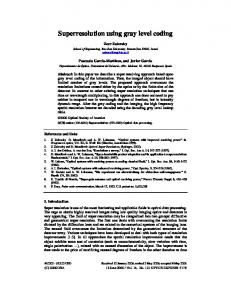
Figure 1. Variational Depth Superresolution using Example-Based Edge Representations. Our method estimates strong edge priors from a given LR depth image and a learned dictionary using a novel sparse coding approach (blue part). The learned HR edge prior is used as anisotropic guidance in a novel variational SR using higher order regularization (red part).
Recent approaches based on learned dictionaries reach a high level of quality for noise free intensity images. However, depth images usually contain higher noise due to sen1
sor characteristics and have fewer high frequency parts. Hence, we propose a method which combines both learning based and SR based on a known PSF. This combination is used in a variational SR together with anisotropic higher order regularization. The whole workflow of our model is depicted in Figure 1. Similar to depth SR approaches that use a high resolution intensity image for guidance we use a sparse coding approach to pre-calculate edge priors out of the low resolution example. The sparse code is reconstructed in a variational energy minimization using a learned dictionary from an external database of low and high resolution examples. In addition to the traditional sparsity constraint we minimize the overlap of neighboring patches in our optimization. This spacial coherence in image space leads to more accurate edges than traditional averaging across the overlap. The edge priors are used as regularization force in a novel variational SR. Hence, our method has the advantage that we do not have to know the exact PSF since the high frequency parts are reconstructed via the edge priors. Furthermore, since we use a variational energy model with Total Generalized Variation (TGV) as regularization we are able to handle depth inputs with higher amounts of noise. In an exhaustive qualitative and quantitative evaluation we show that our methods that combines the advantages of sparse coding and variational SR outperforms current state of the art (SOTA) approaches on multiple real and synthetic datasets.
2. Related Work The field of image superresolution (SR) is a widely researched area in computer vision. While the research on image SR includes also the temporal fusion of multiple acquisitions as well as the combination of different sensor modalities, this work is focused on the SR of single depth images. Therefore, we will limit the related work to recent advances in single image SR based on learned dictionaries and variational SR based on known blur-kernels. We refer interested readers to comprehensive survey papers [17, 27]. Typically, SR approaches based on dictionary learning build upon sparse coding [19]. Yang et al. [28] used the background of sparse coding to reconstruct high resolution test patches as sparse linear combination of atoms from a learned dictionary of paired high and low resolution training patches. Zeyde et al. [30] build upon this framework and improve the quality by adding several modifications. For training they use a combination of K-SVD [1] and Orthogonal Matching Pursuit (OMP) [25] for the low resolution dictionary and a direct regression of the high resolution dictionary using the pseudo-inverse. In the sparse coding approach of Mandal et al. [13] they additional penalized the input and output gradient in each low resolution patch during sparse optimization. Very recently, Timofte et al. [24] accelerated the inference of sparse coding by relaxing the
L0 regularization with L2 regularization and replacing the single dictionary with many smaller sub-dictionaries which are pre-calculated. Hence, finding the sparse representation becomes a quadratic problem for each sub-dictionary which can be solved in closed form. Other works use a dictionary of sample patches in a multi-class labeling problem in a Markov Random Field (MRF). In the work of Freeman and Liu [9] the goal is to minimize the difference of the set of high resolution dictionary atoms to the low resolution input, where the label being optimized represents the high resolution patch. Additionally, the overlap between neighboring patches is penalized in a binary term. Similar, Aodha et al. [12] proposed a MRF framework especially focused on depth image SR with higher noise. In their work an additional depth normalization is proposed to penalize the patch overlap. In a post-processing step they use a novel noise-removal algorithm to increase the quality. Instead of using a dictionary from an external database, Horn´acˇ ek et al. [10] proposed a similar method where the low and high resolution patchpairs of arbitrary size are searched in the image itself. Most methods where the low resolution patches are reconstructed by a combination of dictionary entries highly suffer from input noise as reported in previous works. But there is also a great number of SR approaches that rely on a more general prior, as shown in [17]. Most related to our approach is the variational SR which is based on a known Point Spread Function (PSF) or blur-kernel. Mitzel et al. [15] used this model together with a Total Variation (TV) regularization and optical flow estimation for the image SR of multiple image. This work was extended by Unger et al. [26] proposing a more robust model using the Huber-Norm. In [29] the TV regularization is weighted with an adaptive spatial algorithm based the scene curvature. Our work on depth image SR can be related to both fields since we combine the advances from sparse coding approaches and variational methods based on a known PSF. Compared to previous works, this gives us the possibility to super-resolve depth images with higher amount of noise and where only an approximate blur-kernel is set. Since most man-made environments can be well represented with planar surfaces, we use a Total Generalized Variation (TGV) for regularization which aids the optimization to reconstruct piecewise planar surfaces. This helps to improve on both approaches based on learned dictionaries and on variational SR methods using a known blur-kernel.
3. Superresolution using Sparse Regularization Our approach is focusing on the standard superresolution (SR) problem of recovering a high resolution and highquality depth map Ih ∈ RΩh out of a low resolution and noisy depth map Il ∈ RΩl , where Ωh and Ωl denote the
high and low resolution image space. In our optimization we will rely on the traditional SR reconstruction constraint [29]: An observed low resolution image Il is a blurred and down-sampled version of the noisy high resolution image Ih : Il = DBIh + v,
(1)
where D represents the downsampling operator and B the blur filter. It is assumed that D performs a decimation by a fixed factor and B, representing the blur-kernel, applies a low-pass filter to the image. The additional variable v denotes an unknown amount of noise on the low resolution image. The SR remains extremely ill-posed, since for a given low resolution input Il , infinitely many high resolution images Ih satisfy this reconstruction constraint even if the blur kernel is exactly known. Hence, we utilize the information from an external database of known low and high resolution image pairs to create a useful guidance when solving (1) for Ih . The relationship between low and high resolution images is estimated through the sparsity constraint: For a given low resolution patch the goal is to find the best entry in a dictionary of sample patches collected from an external database of low and high resolution image pairs. Sparse coding approaches aim to overcome this search by using an overcomplete dictionary based on sparse signal representations. Given a learned low resolution dictionary Al the goal is to find the sparse representation α such that the patch is optimally reconstructed by the dictionary entries: pl = Al α,
(2)
n where p √l ∈ R is the low resolution input patch of size √ n × n. The resulting high resolution patch is found through ph = Ah α using the corresponding high resolution dictionary Ah . In section 3.1 we will show a novel approach how to solve (2) densely over the whole image through primal-dual optimization introducing a regularization on the patch overlaps. As a result we get dense edge priors over the whole image. These priors are subsequently used to reconstruct the reconstruction constraint (1), which is shown in 3.2. In section 3.3 we give an overview of the numerical solution of both the sparsity constraint as well as the depth map reconstruction.
3.1. Edge Prior Estimation The goal of the this estimation is to find high resolution edge priors to guide the regularization in a variational superresolution. The estimation of the optimal patch priors for the depth regularization in our model is formulated as finding the best entry in a learned dictionary of sampled patches from low and high resolution image pairs using sparse coding. Similar to most state of the art (SOTA) approaches we
start from the K-SVD dictionary learning of Aharon et al. [1]. Because depth images contain a high variety of discontinuities caused by different scales and sensor modalities we use image features from normalized image patches as low resolution input. Similar to Zeyde et al. [30] we apply PCA dimensionality reduction projecting the features onto an even lower dimensional subspace. Further, we use Orthogonal Matching Pursuit (OMP) [25] to find the sparse code while training. In the training phase we start with a set of low and high resolution image pairs. From these training images we a set of local patch pairs Y = {Yl , Yh } = � create F (pil ), T (psi h ) i extracted at sub-sampled image locations i = {1 . . . p} form Il and si from Ih , where s is the upsampling factor. The operator F (.) : Rn → Rf denotes the feature extraction and dimensionality reduction of the patch pl , where f is the feature length. T (.) : Rn → Rn denotes the calculation of the edge prior out of the high resolution image patch ph . In principle, different kinds of edge priors can be learned in our framework from different kinds of features. In our SR approach we use first and second order gradients as features to learn an anisotropic diffusion edge tensor as described later. After determining the sampled patch pairs, the low resolution dictionary Dl ∈ Rf ×d and the corresponding sparse code Λ ∈ Rd×p = {αi } is found by minimizing min kYl − Dl Λk22 ,
Λ,Dl
s.t.
kΛk0 ≤ L,
(3)
using the K-SVD algorithm, where the size of the dictionary d is fixed. L denotes the number of non-zero entries in the sparse code map Λ. Given Λ the corresponding high resolution dictionary is calculated by the pseudo-inverse ex�−1 pression Dh ∈ Rn×d = Yh ΛT ΛΛT . This is given by the closed form solution of (3) for the dictionary in high resolution space, as shown in [30]. In the reconstruction phase traditional approaches solve (3) through OMP fixing the trained dictionary Dl . The sparse code is estimated for each dictionary atom separately. After reconstruction, the code Λ is multiplied with the high resolution dictionary Dh to get the high resolution patches Yh . These patches are merged and averaged across the image space Ωh to get the resulting image. The downside of this traditional approach of independent calculation and averaging without a neighboring coherence is that the result gets blurry in the overlapping region. This harms the SR quality which is based on the sharpness in the solution, as shown in [12]. In our work we introduce a binary term in the sparse optimization model to introduce spatial coherence of the patches. This enables to reconstruct the sparse code not only with respect to the input patch but also to the difference between neighboring patches. The low resolution
patch is calculated by γ
T (ph ) = exp (−β |∇ph | ) nnT + n⊥ n⊥T ,
Figure 2. Patch-Gradient. The patch-gradient is formulated as the height difference between one patch Dh αi to its direct neighboring patch Dh αi+1 in the image domain. It calculates the pixelwise difference in the overlapping region between two neighboring patches (red area).
patch-features are sparsely reconstructed using the following formulation: min kDl Λ − Yl k22 + λkΛk1 + γk∇p V (Dh Λ)k1 , Λ
(4)
where the first term minimizes the distance of the low resolution dictionary atoms to the input and the second term minimizes the quantity of atoms used for reconstruction. The scalars λ, γ ∈ R weight the individual terms. The L0 constraint of the sparsity constraint is relaxed to a L1 norm constraint, as used in other methods [28]. The additional third term reflects a regularization between overlapping regions of patches. The operator V (.) : Rn×p → Rnp denotes a vectorization of the matrix Dh Λ. The term �T � ∇p = ∇xp , ∇yp : Rnp → R2rp denotes the novel patchgradient operator, where r denotes the size of the overlapping region. Similar to the traditional Total Variation (TV) regularization, the patch-gradient performs absolute forward differences between neighboring patches in x and y direction. For one high resolution patch it is defined as the sum of pixel-wise differences in the overlapping region to its direct neighbor patch in image space.A visualization of this gradient is shown in Figure 2. The patch-gradient penalizer is applied by a simple matrix multiplication of the linear gradient operator ∇p with the concatenated patch vector V (Dh Λ). After optimization we get the concatenated highresolution patches Dh Λ. Since our models finds dictionary entries where the neighbors are better aligned, the resulting image contains sharper edges after merging all the patches back together. In principle, different kinds of the edge priors can be learned in our framework (e.g. scalar weights, image gradients, guided image filters or shock filters). We learn an anisotropic diffusion tensor based on the Nagel-Enkelmann operator [16], since it worked best for all experiments. Given a high resolution depth patch ph the anisotropic edge
(5)
where n is the normalized direction of the image gradient ∇ph n = |∇p , n⊥ is the normal vector to the gradient and the h| scalars β, γ ∈ R adjust the magnitude and the sharpness of the tensor. The gradients are calculated using the Sobel operator to reduce the influence of noise in the training data. The advantage of an anisotropic diffusion tensor is that it not only weights the regularization but also orients the gradient direction during the optimization process, as shown in [21]. This allows for sharper edges across high gradients and prevents high steps along those gradients. In our model the high resolution dictionary is composed of (ideally) incoherent edge tensor entries. After the sparse reconstruction the concatenated tensor entries Dh Λ are merged to the image space resulting in the weighting tensor TΛ ∈ R4×Ωh . This tensor is used in the next step to guide the regularization term in the variational SR.
3.2. Variational Superresolution In the previous section we have shown how to estimate a high resolution edge prior according to a low resolution input image. In this section we propose to solve the SR reconstruction constraint (1) using this prior in a variational energy minimization. The variational SR problem is formulated as min kDBu − Il k� + R(TΛ , u),
(6)
u
where the first term denotes the data fidelity and the second term the regularization R(.) of the optimizer u. In our model, the data term is penalzed by the Huber-Norm [11], defined by ( 2 |x| if |x| ≤ � (7) |x|� = 2� � |x| − 2 if |x| > �. The Huber parameter � ∈ R denotes the tradeoff between the L2 and the L1 norm in the penalization. Hence, the data term gets more robust against Gaussian noise as well as gross outliers in the input depth. Given a fixed upsampling factor s the linear downsampling operator D : RΩh → RΩl is defined by calculating the mean of a pixel region s×s. The formation ofRone pixel fi,j at position (i, j) is calculated as fi,j = s12 ∆s g(x)dx, i,j
with the pixel region ∆si,j = (is, js) + [− 2s , 2s ]2 and g the high resolution image. The quality of traditional SR methods rely on the quality of the blur-kernel, as shown in [14]. In our work we aim to present a more general algorithm where the blur-kernel is not exactly known. The linear blurring operator B : RΩh → RΩh is modeled by a simple Gaussian kernel with a standard
√ deviation σ = 14 s2 − 1 and 3σ for the kernel size. Both linear operators are fixed and can be set in a previous step. In natural environments depth images have less finegrained texture components compared to intensity images. Hence, the regularization term R(.) has to meet the challenges of producing a high resolution depth map that smooths small gradients caused by kernel inaccuracies while preserving strong edges and planar surfaces. Most current regularization terms are based on the TV-norm [18]. This norm favors constant values which causes staircase artifacts in the solution. In our model we use a more general regularization namely the Total Generalized Variation (TGV) [4] of second order. For depth SR this regularization allows to reconstruct piecewise affine surfaces. Together with the learned patch-based edge prior the second order regularizer is formulated as R(TΛ , u) = λ1 kTΛ (∇u − v)k1 + λ0 k∇vk1 ,
(8)
where additionally to the first order smoothness of the depth map, the auxiliary variable v ∈ R2×Ωh is introduced to enforce second order smoothness. The scalars λ0 , λ1 ∈ R are used to weight each order.
3.3. Numerical Optimization In this section we explain the details of the numerical implementation of our method. Both proposed problems are convex but non-smooth due to the L1 and Huber norms in the different terms. Therefore, the optimization of such problems is not a trivial task. Since (4) and (6) are convex in Λ and (u, v) we make use of the dual principle. After introducing Lagrange multipliers for the constraints and biconjugation using the Legendre Fenchel transform (LF) we are able to reformulate the problems as convex-concave saddle point problems, as shown in [3]. Thus, the workflow in our model is defined as first solving the variational sparse coding defined as min maxkDl Λ − Yl k22 + λ hp, Λi Λ
p,q
(9)
+ γ hq, ∇p V (Dh Λ)i . From the resulting sparse code the edge tensor TΛ is estimated by merging the resulting patches Dh Λ into the image space Ωh . The estimated tensor is used in our variational SR approach which is defined as � min max hr, DBu − f i − krk22 u,v r,s,t 2 + λ1 hs, TΛ (∇u − v)i + λ0 ht, ∇vi .
(10)
The matrices p, q, r, s and t denote the introduced dual variables. The feasible sets of all dual variables are defined by a projection onto unit length. Both the sparse coding (9) and the variational SR (10) are solved using the primal-dual optimization scheme, as
proposed by Esser et al. [7]. This scheme provides a fast convergence rate and is parallelized in the implementation resulting in fast optimizations. For a more detailed explanation of the step-by-step algorithm for both optimizations we refer to the supplemental material.
4. Evaluation In this section we show a quantitative and qualitative evaluation of our superresolution (SR) method. We will first discuss some of the algorithm details such as used features and dictionary sizes. Further, we show the performance under acquisition noise where different levels of Gaussian noise are applied on the input data. For an extensive analysis we investigate the performance compared to state of the art (SOTA) approaches on a variety of different datasets including Middlebury [22] and the Laser Scan Dataset of Aodha et al. [12]. For evaluation of the SOTA approaches we use the publicly available framework of Timofte et al. [24]. In the following we compare our method with the standard interpolation methods nearest neighbor (NN) and bicubic upsampling as well as the sparse coding approach of Zeyde et al. [30]. We further show the results of both methods reported in [24], namely Global Regression (GR) and Anchored Neighborhood Regression (ANR), and the neighborhood embedding [2, 5] approaches (NE+LS, NE+NNLS, NE+LLE). Additionally, we compare to the Markov Random Field (MRF) based methods of Aodha et al. [12] and Horn´acˇ ek et al. [10], and the variational SR of Unger et al. [26]1 . For all dictionary based methods we use the same synthetic range image data of [12] for training, which contains 30 scenes of size 800 × 800 in the high resolution space. The reported error is described as the Root Mean Squared Error (RMSE) to a known groundtruth. To allow for a fair comparison all weighting parameters in our model are set once and are kept constant over all experiments. To encourage comparison and future work the results of all reported methods are available at our website.
4.1. Discussion of Algorithm Details For SR based on sparse representations one of the most basic features is to use the sample patches itself. Other methods such as [28, 30, 24] use the first and second order derivative for intensity image features. However, for depth images this is not directly applicable, because the range from minimum to maximum value greatly varies between different scenes. To tackle this problem Aodha et al. [12] proposed a patch normalization which accounts for the ranges of both high and low resolution patch. In our work we first normalize each patch to [0, 1] and then use the 1 Reimplemenation
of the method proposed in [26] for single image SR
(a)
(b)
(c)
Figure 3. Influence of dictionary size and noise on the average RMSE (in pixel disparity) for the Middlebury images Teddy, Cones, Venus and Tsukuba with a magnification of ×3. All neighborhood embedding approaches where used with their best neighborhood size (as reported in [24]). In (a) the results are shown where each sparse coding method uses the same dictionary. In (b) the results for increasing Gaussian noise are shown, where every sparse coding method shares the same dictionary with 1024 entires. In (c) a magnified sector of the noise evaluation in (b) is shown, where the noise level ranges from 0-2% . Figure best viewed magnified in the electronic version.
first and second order gradients as patch-features. An additional PCA dimensionality reduction is applied to project the feature vector onto a lower dimensional subspace while preserving 99.9% of the average energy. For an upscaling factor of 3 this reduces each feature of length 144 to a size of about 36. Throughout all experiments we use a patch-size of 3 × 3 in the low resolution image space, which delivers the best results for all sparse coding approaches. The choice and the size of the dictionary are very critical parts in any sparse coding approach. Usually, the more incoherent atoms a dictionary contains the better the performance, however, this comes with a higher computational cost. In Figure 3a we show the influence of the dictionary size on the performance. As expected, the performance increases with the size of the dictionary. But while the performance of other sparse coding methods drastically increases with the size our method already starts at a much lower RMSE and is less influenced by the choice of the dictionary size. For most depth SR approaches the correct noise handling plays a major role. Therefore, we test the accuracy under different levels of noise on the Middlebury dataset. We chose a depth dependent Gaussian noise with zero mean, as reported in [20]. The standard deviation of the noise ranges from 0 − 50% of the depth range (minimum to maximum) in the input images for an upsampling factor of ×3. In Figure 3b and 3c the error results are shown for the different methods. In Figure 4 we show visual SR results of different methods for a standard deviation of 2%. Obviously, the error increases with the input noise for all methods. But, while the error drastically increases for methods which solely depend on the sparse reconstruction, the variational method [26] produces a higher error at lower noise factors and performs comparably better with increasing noise. This
is caused by the regularization of the depth during optimization which reduces the noise but smooths the edges. Since we use a regularization which is only guided by a sparse edge reconstruction we get more accurate results over the whole noise range.
4.2. Benchmark Evaluation In this section we evaluate the performance of the different SOTA methods on publicly available benchmarks. Following [12, 10] we first show the RMSE results on the Middlebury datasets Teddy, Cones, Venus and Tsukuba for upsampling factors of ×2 and ×4, where the disparity is interpreted as depth. Additionally, we show the results for the real-world laserscan dataset (Scan21, Scan30, Scan42) proposed by [12] for an upsampling factor of ×4. We run our tests on filled ground truth data downscaled by nearest neighbor interpolation (same as used in [12, 10]). The quantitative results are shown in Table 4.1, where we additionally compare our method against SOTA SR methods that use a HR image as guidance [6, 8]. To show the influence of our sparse coding scheme to the overall solution we compare to a combination of the sparse coding method [30] for edge prior estimation in our variational SR ([30] + Our SR). In Figure 5 and 6 the enlarged visual results are shown for an upsampling factor of ×4. The Figures compare the sparse coding approach [30] and the MRF based approaches [12, 10] to our method. Additionally we show the magnitude of the estimated edge prior TΛ which is used as guidance in the SR. What can be clearly seen is that the methods based on a sparse representation have a slightly better performance than the methods based on a MRF or a variational framework. Further, our method that combines both sparse coding and variational SR can still improve on all other methods
×2
×4
×4
Cones
Teddy
Tsukuba
Venus
Cones
Teddy
Tsukuba
Venus
Scan21
Scan30
Scan42
NN Bicubic Diebel and Thrun [6] Ferstl et al. [8]
1.0943 0.9598 0.7397 0.7060
0.8149 0.6917 0.5265 0.5352
0.6123 0.5228 0.4013 0.4412
0.2676 0.2274 0.1703 0.1605
1.5309 1.2386 1.1406 0.9093
1.1292 0.8936 0.8010 0.6267
0.8328 0.6685 0.5490 0.6258
0.3679 0.2938 0.2426 0.1828
0.0177 0.0132 -
0.0163 0.0125 -
0.0396 0.0326 -
Yang et al. [28] Zeyde et al. [30] GR [24] ANR [24] NE+LS NE+NNLS NE+LLE Unger et al. [26] Aodha et al. [12] Horn´acˇ ek et al. [10] Our Method
1.4794 0.6920 0.7780 0.6968 0.7066 0.6886 0.6942 1.1342 1.1269 0.9936 0.6247
1.0909 0.4904 0.5521 0.4954 0.4957 0.6073 0.4995 0.8446 0.8247 0.7910 0.4397
0.8583 0.3871 0.4289 0.3830 0.3939 0.3939 0.3813 0.6445 0.6012 0.5802 0.3504
0.3666 0.1650 0.1896 0.1666 0.1712 0.1646 0.1654 0.2789 0.2761 0.2574 0.1433
1.3239 0.9617 1.0790 1.0050 8.6221 0.9906 0.9766 1.5797 1.5042 1.3986 0.9334
0.9401 0.6953 0.8193 0.7564 10.3913 0.7346 0.7396 1.1131 1.0259 1.1957 0.6670
0.6849 0.5477 0.6480 0.6019 0.5641 0.5704 0.5706 0.8438 0.8333 0.7272 0.4901
0.3010 0.2199 0.2776 0.2452 14.7920 0.2431 0.2406 0.3660 0.3365 0.4501 0.2262
0.0138 0.0100 0.0117 0.0106 0.0818 0.0106 0.0102 0.0170 0.0175 0.0205 0.0085
0.0130 0.0093 0.0114 0.0101 0.1090 0.0101 0.0097 0.0157 0.0170 0.0179 0.0083
0.0337 0.0246 0.0271 0.0264 0.0725 0.0238 0.0262 0.0415 0.0452 0.0299 0.0190
[30] + Our SR
0.6450
0.4543
0.3700
0.1573
0.9430
0.6769
0.4983
0.2363
0.0205
0.0179
0.0299
Table 1. Quantitative evaluation. The RMSE is calculated for different SOTA methods for the Middlebury and the Laserscan dataset for factors of ×2 and ×4. The first four rows show the comparison against two standard interpolation techniques and two depth SR which use an HR intensity image for guidance. The best result of all single image methods for each dataset and upscaling factor is highlighted and the second best is underlined. Additionally we show the sparse coding method [30] used for the edge prior estimation in our SR optimization. The error numbers are given in pixel disparity for the Middlebury and in [mm] for the Laserscan dataset.
both on the synthetic Middlebury dataset and on the realworld laserscan dataset. It can also be seen that for a smaller SR factor of ×2 we get even slightly better results than SOTA intensity image guided approaches since our method does not rely on intensity texture that does not necessarily coincide with depth edges. The visual results point out the differences of the compared methods. The MRF based approaches [12, 10] create sharp edges but miss some important details and suffer from blocking artifacts due to discretization. The sparse coding approach of Zeyde et al. [30] achieves a better accuracy but the result is slightly blurry along sharp edges due to the patch-wise averaging. Our method contains most of the details and reconstructs sharper edges than the sparse coding method but still slightly suffers from the nearest neighbor artifacts. This is visible at very fine details, where the sparse code could not be reconstructed perfectly. Further, it can be seen that the results tends to be over-smoothed at very strong depth discontinuities, because the magnitude of the anisotropic tensor is proportional to the depth gradient.
4.3. Conclusion In this work we propose a method for single depth image superresolution. The algorithm is designed in two steps. First, edge priors are estimated using sparse coding with a learned dictionary out of high and low resolution patch pairs. Second, the learned edge priors are used in variational energy minimization using a higher order Total Generalized Variation regularization. With this combination we are able to get more robust against noise than state of the art sparse
coding approaches and more accurate than variational approaches where the exact blur kernel has to be known. In a quantitative and qualitative evaluation using widespread datasets we show that our method qualitatively outperforms existing methods. To cope with non-valid pixels in the input (occlusions for stereo depth) our method can be easily extended by a weighting parameter of the SR data term, which is zero for non-valid and one for valid pixels. As the proposed method is not limited to single image superresolution we plan to incorporate a temporal coherence using existing scene flow methods. This will eventually lead to an even higher accuracy.
Acknowledgments This work was supported by Infineon Technologies Austria AG, the Austrian Research Promotion Agency (FFG) under the FIT-IT Bridge program, project #838513 (TOFUSION).
References [1] M. Aharon, M. Elad, and A. Bruckstein. K-svd: An algorithm for designing overcomplete dictionaries for sparse representation. Trans. Sign. Proc., 54(11):4311–4322, Nov 2006. 2, 3 [2] M. Bevilacqua, A. Roumy, C. Guillemot, and M. line Alberi Morel. Low-complexity single-image super-resolution based on nonnegative neighbor embedding. In BMVC, 2012. 5 [3] S. Boyd and L. Vandenberghe. Convex Optimization. Cambridge University Press, 2004. 5
(a) Noisy input
(b) Zeyde et al. [30]
(c) NE-NNLS
(d) Unger et al. [26]
(e) OURS
(f) Tensor TΛ
Figure 4. Color-coded visual SR results for noisy input data. The figure shows a zoomed region of interest from the Teddy dataset for an upsampling factor of ×3. On the low resolution input we applied Gaussian noise with zero mean and a standard deviation of 2% of the input disparity range. Figure best viewed magnified in the electronic version.
(a) Groundtruth
(b) Zeyde et al. [30]
(c) Aodha et al. [12]
(d) Horn´acˇ ek et al. [10]
(e) OURS
(f) Tensor TΛ
Figure 5. Color-coded Middlebury results. The figure shows a zoomed region of interest from the Cones (first row) and the Tsukuba (second) example form the Middlebury dataset for an upsampling factor of ×4. Figure best viewed magnified in the electronic version.
(a) Groundtruth
(b) Zeyde et al. [30]
(c) Aodha et al. [12]
(d) Horn´acˇ ek et al. [10]
(e) OURS
(f) Tensor TΛ
Figure 6. Color-coded Laserscan results. In the figure zoomed regions of interest from the Scan21 dataset of Aodha et al. [12] are shown for an upsampling factor of ×4. Figure best viewed magnified in the electronic version.
[4] K. Bredies, K. Kunisch, and T. Pock. Total generalized variation. SIAM Journ. on Imag. Sciences, 3(3):492– 526, 2010. 5 [5] H. Chang, D.-Y. Yeung, and Y. Xiong. Super-resolution through neighbor embedding. In CVPR, June 2004. 5 [6] J. Diebel and S. Thrun. An application of markov random fields to range sensing. In NIPS, 2006. 6, 7 [7] E. Esser, X. Zhang, and T. Chan. A general framework for a class of first order primal-dual algorithms for convex optimization in imaging science. SIAM Journ. on Imag. Sciences, 3(4):1015 –1046, 2010. 5 [8] D. Ferstl, C. Reinbacher, R. Ranftl, M. R¨uther, and H. Bischof. Image guided depth upsampling using anisotropic total generalized variation. In ICCV, 2013. 1, 6, 7 [9] B. Freeman and C. Liu. Markov random fields for superresolution and texture synthesis. In In: Advances in Markov Random Fields for Vision and Image Processing. MIT Press, 2011. 2 [10] M. Horn´acˇ ek, C. Rhemann, M. Gelautz, and C. Rother. Depth super resolution by rigid body self-similarity in 3d. In CVPR, 2013. 2, 5, 6, 7, 8 [11] P. J. Huber. Robust regression: Asymptotics, conjectures and monte carlo. Annal. of Stat., 1(5):799 –821, 1973. 4 [12] O. Mac Aodha, N. D. Campbell, A. Nair, and G. J. Brostow. Patch based synthesis for single depth image superresolution. In ECCV, 2012. 2, 3, 5, 6, 7, 8 [13] S. Mandal, A. Bhavsar, and A. Sao. Hierarchical examplebased range-image super-resolution with edge-preservation. In ICIP, 2014. 2 [14] T. Michaeli and M. Irani. Nonparametric blind superresolution. In ICCV, 2013. 4 [15] D. Mitzel, T. Pock, T. Schoenemann, and D. Cremers. Video super resolution using duality based tv-l1 optical flow. In DAGM, 2009. 2 [16] H.-H. Nagel and W. Enkelmann. An investigation of smoothness constraints for the estimation of displacement vector fields from image sequences. TPAMI, 8(5):565 –593, 1986. 4 [17] K. Nasrollahi and T. Moeslund. Super-resolution: a comprehensive survey. MVA, 25(6):1423–1468, 2014. 2 [18] M. Nikolova. A variational approach to remove outliers and impulse noise. Journal of Mathematical Imaging and Vision, 20(1-2):99 –120, 2004. 5 [19] B. A. Olshausen and D. J. Field. Sparse coding with an overcomplete basis set: A strategy employed by v1? Vision Research, 37(23):3311 –3325, 1997. 2 [20] J. Park, H. Kim, Y.-W. Tai, M. Brown, and I. Kweon. High quality depth map upsampling for 3d-tof cameras. In ICCV, 2011. 6 [21] C. Reinbacher, T. Pock, C. Bauer, and H. Bischof. Variational segmentation of elongated volumetric structures. In CVPR. 4 [22] D. Scharstein and R. Szeliski. High-accuracy stereo depth maps using structured light. In CVPR, 2003. 5 [23] S. Schuon, C. Theobalt, J. Davis, and S. Thrun. Lidarboost: Depth superresolution for tof 3d shape scanning. In CVPR, 2009. 1
[24] R. Timofte, V. De Smet, and L. Van Gool. Anchored neighborhood regression for fast example-based super-resolution. In ICCV, 2013. 2, 5, 6, 7 [25] J. Tropp and A. Gilbert. Signal recovery from random measurements via orthogonal matching pursuit. Trans. Information Theory, 53(12):4655–4666, Dec 2007. 2, 3 [26] M. Unger, T. Pock, M. Werlberger, and H. Bischof. A convex approach for variational super-resolution. In DAGM, 2010. 1, 2, 5, 6, 7, 8 [27] J. van Ouwerkerk. Image super-resolution survey. Image and Vision Computing, 24(10):1039 –1052, 2006. 2 [28] J. Yang, J. Wright, T. Huang, and Y. Ma. Image superresolution via sparse representation. Trans. Imag. Proc., 19(11):2861–2873, 2010. 2, 4, 5, 7 [29] Q. Yuan, L. Zhang, and H. Shen. Multiframe superresolution employing a spatially weighted total variation model. Trans. CSVT, 22(3):379–392, 2012. 2, 3 [30] R. Zeyde, M. Elad, and M. Protter. On single image scale-up using sparse-representations. In Curves and Surfaces, volume 6920, pages 711–730. 2012. 1, 2, 3, 5, 6, 7, 8