Variational Bayesian Image Restoration Based on a Product of t ...

IEEE TRANSACTIONS ON IMAGE PROCESSING, VOL. 17, NO. 10, OCTOBER 2008

1795

Variational Bayesian Image Restoration Based on a Product of t-Distributions Image Prior Giannis Chantas, Nikolaos Galatsanos, Aristidis Likas, and Michael Saunders

Abstract—Image priors based on products have been recognized to offer many advantages because they allow simultaneous enforcement of multiple constraints. However, they are inconvenient for Bayesian inference because it is hard to find their normalization constant in closed form. In this paper, a new Bayesian algorithm is proposed for the image restoration problem that bypasses this difficulty. An image prior is defined by imposing Student-t densities on the outputs of local convolutional filters. A variational methodology, with a constrained expectation step, is used to infer the restored image. Numerical experiments are shown that compare this methodology to previous ones and demonstrate its advantages. Index Terms—Constrained variational inference, image restoration, product prior, Student’s-t prior, Variational Bayesian Inference.

I. INTRODUCTION

I

MAGE restoration is a well known ill-posed inverse problem that requires regularization. Regularization based on Bayesian methodology is very popular since it provides a systematic and rigorous framework for estimation of the model parameters. Regularization in a Bayesian framework corresponds to the introduction of a prior for the image statistics [1], which enforces prior knowledge for the image. Initially, stationary Gaussian priors were used; see for example [2] and [3]. Such priors are convenient from an implementation point of view because they require only one parameter; however, they have the drawback of not being able to preserve edges and they smooth noise in flat areas of the image. To avoid this problem, there has been a very large body of work in the last 20 years. A number of methods have been introduced to regularize in a spatially variant manner, or equivalently, many edge-preserving priors have been proposed. A detailed survey on this topic is beyond the scope of this paper. In what follows, we selectively reference work that is pertinent to the herein proposed approach. Manuscript received January 7, 2008; revised June 7, 2008. Current version published September 10, 2008. This work was supported in part by the E.U.European Social Fund (75%) and in part by the Greek Ministry of DevelopmentGSRT (25%). The associate editor coordinating the review of this manuscript and approving it for publication was Dr. Michael Elad. G. Chantas and A. Likas are with the Department of Computer Science, University of Ioannina, Ioannina, Greece, 45110 (e-mail: [email protected]; [email protected]). N. Galatsanos is with the Department of Electrical and Computer Engineering, University of Patras, Rio, 26500, Greece (e-mail: [email protected]). M. Saunders is with the Department of Management Science and Engineering (MS&E), Stanford University, Stanford, CA USA 94305-4026 (e-mail: [email protected]). Digital Object Identifier 10.1109/TIP.2008.2002828

Priors based on robust Huberov statistics and Generalized Gaussian pdfs have also been used; see, for example, [4] and [5]. Recently, such a prior was used along with the majorization minimization framework to derive an edge-preserving image restoration algorithm that can be implemented very efficiently using the fast Fourier transform [6]. The main shortcomings of such priors are that their normalization constant is hard to find. The parameters of such models have to be adjusted empirically. Another class of algorithms, which have been very popular in certain image processing circles designed for edge-preserving restoration, is based on the total variation (TV) criterion [8]. Although TV-based regularization has been popular, till recently it involved ad hoc selection of certain parameters. Recently, though, a Bayesian framework was proposed that allows estimation of these parameters in a rigorous manner. Nevertheless, improper priors were used in these works, and as a result these methodologies contain an element of subjective selection [9], [10] and [11]. Priors based on wavelet decompositions and heavy-tailed pdfs have been used for edge-preserving image restoration in [12] and [13] along with the EM algorithm. In [7] and [14], the denoising problem was addressed with heavy-tailed priors in the wavelet domain. Image denoising involves a simpler imaging model; as a result Bayesian inference is easier in this case. A Gaussian scale mixture (GSM) was used to model the wavelet coefficients in [7] and a one-step algorithm for inference. In [14], Hirakawa and Meng used the Student-t pdf to model the statistics of the wavelet coefficients, and derived an EM algorithm for inference. The Student’s-t pdf is a special case of a GSM. Product-based image priors have also been proposed in [15]. Such priors combine in product form multiple probabilistic models. Each individual model gives high probability to data vectors that satisfy just one constraint. Vectors that satisfy only this constraint but violate others are ruled out by their low probability under the other terms of the product model. Image priors based on this idea have been used in image recovery problems [15] and [16]. However, such priors were learned using a large training set with images and stochastic sampling methods and used in a number of image recovery problems based on “empirical” maximum a posteriori approaches and gradient descent minimization [15]. This differs from the herein proposed approach where the product prior is learnt only from the observations. The term “empirical” is used because the PoE priors used were not normalized; thus, the parameters of the recovery algorithm cannot be estimated or inferred rigorously but were adjusted rather empirically. In [17], [18], and [19], some of us proposed a new hierarchical image prior for image restoration, image super-resolution, and

1057-7149/$25.00 © 2008 IEEE Authorized licensed use limited to: Illinois Institute of Technology. Downloaded on January 21, 2009 at 23:34 from IEEE Xplore. Restrictions apply.

1796

IEEE TRANSACTIONS ON IMAGE PROCESSING, VOL. 17, NO. 10, OCTOBER 2008

blind image deconvolution problems, respectively. This prior is Student-t based, is in a product form, and is able to capture the local image discontinuities and thus provide edge-preserving capabilities for those problems. Its main shortcomings are that both the normalization constant and the hyper-parameters of the prior were found heuristically. Furthermore, image models based on Student-t statistics have been used with success in other than image reconstruction applications. For example, in [21], such models were used with success for watermark detection. Inspired by our previous work, we now propose a new Bayesian inference framework for image deconvolution using a prior in product form. This prior assumes that the outputs of local high-pass filters are Student-t distributed. The main contribution of this work is a Bayesian inference methodology that bypasses the difficulty of evaluating the normalization constant of product type priors. The methodology is based on a constrained variational approximation that uses the outputs of all the local high pass filters to produce an estimate of the original image. More specifically, a constrained expectation step is used to capture the relationship of the filter outputs of the prior to the original image. In this manner, the use of improper priors is avoided and all the parameters of the prior model are estimated from the data. Thus, the “trial and error” parameter “tweaking” required in [17]–[19] and other state-of-the-art recently proposed restoration algorithms, which makes their use difficult use for nonexperts, is avoided. Furthermore, the proposed restoration algorithm provides competitive performance compared with previous methods. In this work, we also propose an efficient Lanczos-based computational framework tailored to the calculations required in our Bayesian algorithm. More specifically, a very large linear system is solved iteratively and the diagonal are simultaneously estimated in elements of a matrix an efficient manner. The rest of this paper is organized as follows. In Section II, the imaging and image model are defined. In Section III, the variational restoration algorithm is derived. In Section IV, we present the computational methodology used to implement our algorithm. In Section V, numerical experiments are demonstrated. Finally, Section VI gives conclusions and thoughts for future work. II. IMAGING AND IMAGE MODEL A. Imaging Model A linear imaging model is assumed. For convenience but without loss of generality, we use 1-D notation. The vector represents the observed degraded image obtained by (2.1) known where is the (unknown) original image, is an convolution matrix and is additive white noise. We assume Gaussian statistics for the noise given by where is an vector of zeros, is the identity matrix and is the noise precision (inverse variance), which is assumed unknown.

Aiming at the definition of the image prior we first define operators for and use them to define filter outputs (2.2) . The matrices repwhere resenting the operators are of size and the filter outputs are of size . These operators are zero mean convolutional high-pass filters and each one of them is used to impose a particular constraint on the restored image. B. Image Prior Model We assume that for Student-t distributed, with parameters

are i.i.d zero mean and (2.3)

where

The Student-t implies a two-level generation process [22]. is first drawn from a Gamma disMore specifically, tribution, . Then, is generated from a zero-mean Normal distributhe , according to tion with precision . The probability density function of (2.3) can be written as an integral

The variables are called “hidden” (latent) because they are not apparent in (2.3), since they have been integrated out. There are two extremes in this generative model, depending on the value of the “degree of freedom” parameter . As this ’s are parameter goes to infinity, the pdf from which the drawn has its mass concentrated around 1. This in turn reduces are the Student-t to a Normal distribution, because all drawn from the same Normal with precision , since . The other extreme is when and the prior becomes uninformative. In general, for small values of the probability mass of the Student-t pdf is spread, rendering the Student-t more “heavy-tailed”. The use of heavy-tailed priors on high-pass filters of the image is a characteristic of most modern “edge preserving” image priors used for regularization in a stochastic setting; see for example [4]–[6], [11], [14], [15], and [19]. The main idea behind this assumption is that at the few edge areas of an image will be large in absolute value. Thus, it the filter outputs is important to model them with a heavy-tailed pdf in order to allow the prior to encourage formation of edges. The downside

Authorized licensed use limited to: Illinois Institute of Technology. Downloaded on January 21, 2009 at 23:34 from IEEE Xplore. Restrictions apply.

CHANTAS et al.: VARIATIONAL BAYESIAN IMAGE RESTORATION BASED ON A PRODUCT OF -DISTRIBUTIONS IMAGE PRIOR

of many such models is that most heavy-tailed pdfs are not amenable to Bayesian inference. For example, the Generalized Gaussian and the Alpha Stable pdfs can be also heavy tailed. However, unlike the Student-t where Bayesian inference is possible [27], moment-based estimators have to be used for their parameters; see for example [24] and [25]. . We now define the following notation for the variables We denote by a vector, where . Also, for the filter outputs we use . We assume that the notation the filter outputs are independent not only in each pixel location but also in each direction. This assumption makes subsequent calculations tractable. Thus, the cumulative density for the filter outputs conditioned on is (2.4) where and is a diagonal matrix with elements the components of the vector . At this point, the marginal distribution yearns for a closed form, using the relation between the image and the filter outputs, (2.2). However, this prior is analytically intractable because one cannot find in closed form its normalization constant. This problem stems from the fact that it is not possible because to find the eigenvalues of the matrix does not have a it is very large and the product structure that is amenable to efficient eigenvalue computation. One contribution of this work is that we bypass this difficulty by exploiting the commuting property of convolutional operators and derive a constrained variational algorithm for approximate Bayesian inference. This algorithm is described in detail next. III. VARIATIONAL ALGORITHM Since, as explained above, it is difficult to infer a solution for the image from the Bayesian model previously defined, a transformed imaging model is introduced in Section 3.1.

1797

. For this reason, we must initially define the posterior of the observations given . This is equal to the product of Normal distributions, since the observations are assumed indepedent :

The prior for the residuals has been already defined in (2.3). Working in the Bayesian framework, we define as latent (hidden) variables the residuals and the inverse variances . Hence, the complete data likelihood is

where . Estimation of the model parameters ideally could be obtained through maximization of the marginal distribution of the observations (3.3) However, in the present case, this marginalization is not possible. Furthermore, since the posterior of the hidden variables is not known explicitly, infergiven the observations ence via the Expectation-Maximization (EM) algorithm is not possible [29]. For this reason, we resort to the variational methodology [22], [28] and [29]. According to this methodology, we introduce a lower bound on the logarithm of the marginal likelihood, which is actually the expectation of the logarithm of the complete data likelihood with respect to an auxiliary function of the hidden minus the entropy of variables

A. Variational Algorithm for the Equivalent Imaging Model The imaging model of (2.1) can be written as (3.1) (3.4) Setting for and using (2.2), we can utilize the commuting property of the convolutional operators and write the imaging model as (3.2) where are the observations of the newly defined model and the additive noise is

The inequality holds because the functional is also equal to the logarithm of the marginal likelihood minus the always nonnegative Kullback–Leibler divergence between the true posteof the hidden variables and ; rior distribution see for example [22]. , or equivEquality holds in (3.4) when alently (3.5)

In this model, we assume that the filter outputs of our filters are the unknowns. Thus, the algorithm will infer instead of . In this manner we bypass the need to define a prior for

because in this case the Kullback–Leibler divergence becomes zero.

Authorized licensed use limited to: Illinois Institute of Technology. Downloaded on January 21, 2009 at 23:34 from IEEE Xplore. Restrictions apply.

1798

IEEE TRANSACTIONS ON IMAGE PROCESSING, VOL. 17, NO. 10, OCTOBER 2008

In the variational Bayesian framework, instead of maximizing the unobtainable marginal likelihood, we maximize the bound , (3.4), with respect to both and in the variational E and M steps, respectively. In other words, the unknown posterior is approximated by . One difficulty in this is hard approach is that the maximization with respect to to obtain in closed form, although we can bypass it by using the so-called Mean Field approximation [29]. According to this approximation, if we assume that

This is achieved by iterating between the two following steps, is the iteration index: where

(3.6) then unconstrained optimization of the functional with respect to all yields Normal distributions (3.7) and . The difficulty that we encounter with the above posteriors, which were obtained by unconstrained optimization, is that they do not provide a method to infer from , and they do not capture their common origin from , (2.2). In order to bypass this difficulty we make the assumption is Normal; however, it is conthat each of the posteriors strained so that it captures the common origin of all from , as dictated by (2.2). In other words, we assume that with parameters

Thus, in the E-step of the variational algorithm, optimization of the functional is performed with respect to the auxiliary functions. However, in the present case, the functions , are assumed to be Normal distributions with partially common mean and covariance [see (3.8)]; therefore, this bound and and a funcis actually a function of the parameters tional w.r.t. the auxiliary function . Using (3.6), the variational bound in our problem becomes

(3.9) (3.8) where and are actually parameters representing the mean originate. In and covariance of the image , from which all other words

Thus, and are parameters that are used in our model and estimated during the restoration algorithm. Actually, the restored image is taken to be the estimate of .

where and . Thus, in the VE-step of our algorithm the bound must be optiand mized with respect to

Taking the derivative of w.r.t to and (see Appendix), we find that the bound is maximized w.r.t. these parameters when

(3.10)

B. Variational Update Equations The general variational algorithm using the Mean Field approximation [29] for approximate inference of a statistical model with as observation, hidden variables and parameters denoted by , aims to maximize the bound

(3.11)

(3.12) where that since each

and . Notice is a Gamma pdf of the form

Authorized licensed use limited to: Illinois Institute of Technology. Downloaded on January 21, 2009 at 23:34 from IEEE Xplore. Restrictions apply.

CHANTAS et al.: VARIATIONAL BAYESIAN IMAGE RESTORATION BASED ON A PRODUCT OF -DISTRIBUTIONS IMAGE PRIOR

, its expected value is

(3.13) where denotes the expectation w.r.t. an arbitrary distri. This is used in (3.10) and (3.11), where is a bution diagonal matrix with elements

At the variational M-step the bound is maximized with respect to the model parameters

where is calculated using the results from (3.10)–(3.13). The update for is obtained after taking the derivative and equating to zero

(3.14) In the same way, the maximum is attained for

(3.15) Finally, taking the derivative with respect to and equating to zero, we find the “degrees of freedom” parameter of the Student-t by solving the equation

1799

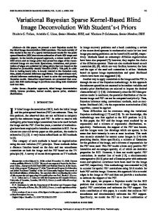
IV. COMPUTATIONAL IMPLEMENTATION In our implementation, the variance of the additive noise is estimated in a preprocessing step and is kept fixed. The EM algorithm with a stationary Gaussian prior [3] and one output (the Laplacian operator) was used for this purpose. Furthermore, the EM-restored image was used to initialize our algorithm. For all were used for the prior. experiments, four filter outputs We show the magnitude of the frequency responses of these filand correspond to the horiters in Fig. 2. The operators zontal and vertical first order differences. Thus, these filters are used to model the vertical and horizontal image edge structure, and are used to respectively. The other two operators model the diagonal edge component contained in the vertical and horizontal edges, respectively. These filters are obtained by convolving the previous horizontal and vertical first order differences filters with fan filters with vertical and horizontal pass-bands, respectively. In our experiments, the fan filters in [26] were used. We solve (3.10) and (3.16) iteratively. For (3.16), we employ the bisection method, as also proposed in [27]. In the next few paragraphs, we analyze how (3.10) is solved by a method based on the Lanczos process [29], [30]. Omitting the subscripts and superscripts for convenience, we regard (3.9) as the linear system , where is symmetric and positive definite, , can be obtained efficiently for any given . and products In addition, we have the linear algebra problem of estimating in (3.13). The matrix the diagonals of matrix is very large; for example for 256 256 images it is with and clearly an iterative of dimension method must be used. The Lanczos process is an iterative procedure for transforming to tridiagonal form [32]. Given some starting vector , it generates vectors and scalars as follows. (meaning and but 1. Set exit if ). set 2. For . After steps, the situation can be summarized as (4.1)

..

(3.16) for

, where

is the digamma function and is the value of at the preused to evaluate the expectations in (3.13) vious iteration during the VE-step.

.

..

.

..

.

(4.2)

where is the th unit vector, has theoretically orthonormal columns, and is tridiagonal and symmetric. In unless is reorthogonalized with practice, respect to previous vectors, but relation (4.1) remains accurate and to be used to to machine precision. This permits solve accurately in a manner that is algebraically equivalent to the conjugate-gradients method, as described in [30] (It also leads to reliable methods for solving when is indefinite [30]). Note that must be proportional to as shown.

Authorized licensed use limited to: Illinois Institute of Technology. Downloaded on January 21, 2009 at 23:34 from IEEE Xplore. Restrictions apply.

1800

IEEE TRANSACTIONS ON IMAGE PROCESSING, VOL. 17, NO. 10, OCTOBER 2008

TABLE I ISNR RESULTS COMPARING THE PROPOSED ALGORITHM WITH THE ALGORITHMS IN [9], [10], AND [11] USING THREE IMAGES, THREE NOISE LEVELS, AND GAUSSIAN SHAPED BLUR. THE ISNR RESULTS FOR THE BFO1, BFO2, BMK1, AND BMK2 ALGORITHMS ARE OBTAINED FROM [11]

When is positive definite, each is also positive definite (with and we may form the Cholesky factorization lower-triangular) by updating . The conjugate-gradient method computes a sequence of approximate solutions to in the form , where is defined by the equation . Since exactly for all n, we , where the residual vector see from (4.1) that becomes small if either is small (unlikely in practice) or the last element of is small. itself because every elIn practice, we do not compute . Instead, we compute two quantities ement differs from and by applying forward substitution to the lower-triangular systems and , where

(4.3)

can be updated according to . Since is bidiagonal, only the most need to be retained in memory. Thus, recent columns of the previous equation is the update rule for the image estimate in the algorithm. , we can make use of the In order to estimate elements of in (4.3). If we now assume that exact arithmetic same vectors holds, we see that so that

If we further assume that the Lanczos process continues for iterations, we have , so that . , we have the seOn this basis, if we define . To estiquence of estimates . mate its th diagonal, we form the sum

Authorized licensed use limited to: Illinois Institute of Technology. Downloaded on January 21, 2009 at 23:34 from IEEE Xplore. Restrictions apply.

CHANTAS et al.: VARIATIONAL BAYESIAN IMAGE RESTORATION BASED ON A PRODUCT OF -DISTRIBUTIONS IMAGE PRIOR

1801

TABLE II ISNR RESULTS COMPARING THE PROPOSED ALGORITHM WITH THE ALGORITHMS IN [9], [10], AND [11] USING THREE IMAGES, THREE NOISE LEVELS, AND UNIFORM BLUR. THE ISNR RESULTS FOR THE BFO1, BFO2, BMK1, AND BMK2 ALGORITHMS ARE OBTAINED FROM [11]

Thus, we can obtain monotonically increasing estimates for all diagonals at very little cost,1 in the manner of LSQR [33]. Similarly, for the matrix , whose diagonals we wish to estimate, we have

where can be formed at each Lanczos iteration and then discarded after use. This is how we evaluate in (3.12). Element estimation of inverses of large matrices is also required in many other recently developed Bayesian algorithms 1See http://www.stanford.edu/group/SOL/software/cgLanczos.html Matlab code.

(see for example [11], [19], and [23]) and presently to the best of our knowledge are handled either by inaccurate circulant or diagonal approximations of the matrix or by very time-consuming Monte-Carlo approaches. An iteration of the variational EM algorithm consists of the update steps given by (3.9)–(3.12) and (3.14)–(3.15). In our implementation, the parameter is estimated in a preprocessing step, as described above. During the variational M-step the bisection method is used for the update of the parameters with , where is the termination criterion at the th iteration of the bisection method. The value of linear system in (3.10) is solved by the iterative Lanczos procedure. The termination criterion for this algorithm is

for

Authorized licensed use limited to: Illinois Institute of Technology. Downloaded on January 21, 2009 at 23:34 from IEEE Xplore. Restrictions apply.

1802

IEEE TRANSACTIONS ON IMAGE PROCESSING, VOL. 17, NO. 10, OCTOBER 2008

2

Fig. 1. (a) Degraded “Cameraman” image by uniform 9 9 blur and noise with BSNR = 40 dB, (b) restored image using a stationary Gaussian prior [3] ISNR = 4:57 dB, (c) restored image using TV TE ISNR = 9:07 dB, (d) restored image using proposed algorithm ISNR = 9:53 dB.

0

where denotes the iteration index of the Lanczos process (hence, ). Thus, is the image estimate at the -th Lanczos iteration and at the -th iteration of the overall denotes the Frobenius variational algorithm. Lastly, norm. As criterion for termination of the variational algorithm . In other words, we terminate we used the overall algorithm when the residual of the Lanczos process is larger than that of the iteration . at iteration The overall algorithm is summarized in the following threestep procedure. using a stationary model [3]. 1. Initialize 2. Repeat until convergence: -th iteration: and using (3.10), • VE-step: Update, (3.12) and (3.13), respectively. For the last equation, and also need to be calculated. Also, calculate from (3.13), need for the the expected value of th iteration. VM-step and the next VE-step in the using (3.15) and by solving • VM-step: Update (3.16) for each . as the restored image estimate. 3. Use V. NUMERICAL EXPERIMENTS We demonstrate the value of the proposed restoration approach by showing results from various experiments with

three 256 256 input images: “Lena,” “Cameraman,” and “Shepp–Logan” phantom. Every image is blurred with two types of blur; the first has the shape of a Gaussian function with shape parameter 9, and the second is uniform with support a rectangular region of 9 9 pixels. The blurred signal to noise ratio (BSNR) defined as follows was used to quantify the noise level:

where is the variance of the additive white Gaussian noise (AWGN). Three levels of AWGN were added to the blurred im40, 30, and 20 dB. Thus, in total 18 image ages with restoration experiments were performed to test the proposed algorithm. As performance metric, the improvement in signal-to-noise ratio (ISNR) was used

where and are the original, observed degraded and restored images, respectively. We present ISNR results comparing our algorithm with four total-variation (TV) based Bayesian algorithms in [10] abbreviated as BFO1, in [9] abbreviated as BFO2, and [11] abbreviated

Authorized licensed use limited to: Illinois Institute of Technology. Downloaded on January 21, 2009 at 23:34 from IEEE Xplore. Restrictions apply.

CHANTAS et al.: VARIATIONAL BAYESIAN IMAGE RESTORATION BASED ON A PRODUCT OF -DISTRIBUTIONS IMAGE PRIOR

Q ), (b) vertical differences (Q ), (c) Q

Fig. 2. Magnitude of frequency responses of the filters used in the prior: (a) horizontal differences (

1803

and (d)

Q.

TABLE III ISNR RESULTS COMPARING THE PROPOSED ALGORITHM WITH THE ALGORITHMS IN [9] USING 3 IMAGES, 3 NOISE LEVELS AND BLUR [1 4 6 4 1] [1 4 6 4 1]=256

as BMK1 and BMK2. For comparison purposes we also implemented a restoration algorithm based on TV regularization [8]. with respect to the This algorithm minimizes the function image

where and are the directional differences vectors of the image along the horizontal and vertical direction respectively. A conjugate gradient algorithm is used to minimize with a one-step-late quadratic approximation [8]. The parameters and were kept fixed during the iterations of this algorithm and were selected by trial-and-error (TE) to optimize ISNR assuming knowledge of the original image. Since this algorithm assumes knowledge of the original it is not a realistic one. However, it provides the performance bound of the TV algorithm with fixed parameters. In Tables I and II, we present ISNR results comparing our algorithm with the above-mentioned methods in 18 experiments. The ISNR results for BFO1, BFO2, BMK1, and BMK2 were obtained from [11]. In these tables for reference purposes we also provide ISNR results for the stationary simultaneously autoregressive prior in [3]. In Fig. 1, restoration results are shown for the “Cameraman” dB noise and uniform blur. In this image with experiment the restored image by the proposed algorithm is superior in ISNR, and is visually distinguishable from the TV-TE approach, which was optimized using the original image.

At this point we note that the proposed algorithm performed very well compared with the TV-based methods in [9], [10], dB case it and [11]. More specifically, for the high gave the best results from all methods (excluding TV-TE since it is unrealistic) in 5 out of 6 experiments. For the midlevel dB case it gave the best performance in 5 out of 6 experiments. Finally, in the low dB case it gave the best result in 3 out of the 6 experiments. Overall the proposed algorithm gave the best ISNR results in 13 out of 18 experiments, compared to 3 out of 18 for BFO1 and 2 out of 18 for BFO2. We also compared our method with BFO1 [9], which based on the above experiments was the most competitive TV based method. We used the same three images and noise levels as above. We also used a 5 5 pyramidal blur with impulse re. The ISNR results sponse given by for this experiment are given in Table III. For the implementation we used the code provided by the authors.2 The ISNR results from this experiment are consistent with the previous ones. VI. CONCLUSIONS AND FUTURE RESEARCH We presented a new Bayesian framework for image restoration that uses a product-based Student-t type of priors. The main theoretical contribution is that by constraining the approximation of the posterior in the variational framework, we bypass the need for knowing the normalization constant of this 2http://www.lx.it.pt/~jpaos

Authorized licensed use limited to: Illinois Institute of Technology. Downloaded on January 21, 2009 at 23:34 from IEEE Xplore. Restrictions apply.

1804

IEEE TRANSACTIONS ON IMAGE PROCESSING, VOL. 17, NO. 10, OCTOBER 2008

prior. Thus, we avoid having to use improper priors, i.e., priors whose normalization constant is empirically selected; see, for example, [9]–[11], [17], [18], and [19]. Furthermore, the proposed methodology does not require empirical parameter selection as in the MAP methodology that uses a similar-in-spirit prior in [17] and [18]. We also presented a Lanczos-based computational scheme tailored to the computations required by our algorithm. We demonstrated by the ISNR results in Tables I–III that the proposed method is competitive with the very recently proposed TV-based Bayesian algorithms in [9], [10], and [11]. More specifically, it appears that this approach is more competitive in the higher BSNR cases. Thus, it seems that in such cases the proposed Student-t model has the ability to capture more accurately than TV-based priors subtle features of the image present in the observations. However, in the presence of high levels of AWGN this does not seem to be the case and the advantage of our proposed prior compared to TV priors seems to diminish. We believe that this is the case because high levels of noise “wipe out” the subtle features that our model can capture. We found empirically that modeling explicitly the diagonal edge structure contained in the vertical and horizontal edge (the and ) improved the performance of the use of operators proposed algorithm, for a wide range of images, blurs and SNRs. Selecting optimally such operators according to the image is a topic of current investigation. Another topic of current investigation is image models that capture the spatial correlation between the outputs of the convolutional filters used in the prior. We plan to address this point by assuming a similar-in-spirit prior that uses a neighborhood around each pixel and multidimensional Student-t pdfs. Another point that we plan to investigate is the use of generalized Student-t pdfs. These pdfs depend on and the “classical” Stu. dent-t used herein is just a special case with

Because at this point we aim to optimize with respect to , we operate on the function , which includes only the terms that depend on the parameters

(A.1) The first sum is further analyzed

(A.2) where

is a diagonal matrix with elements

The second integral is the entropy of a Gaussian function, which is proportional to

APPENDIX In the VE-step the bound must be optimized with respect to and . With the mean field approximation (3.6) the bound becomes

where

and

.

(A.3) Setting the derivative of w.r.t equal to zero using (A.1)–(A.3) yields the equation shown at the bottom of the page. Similarly, using (A.2), we find that the optimum for the mean

The final part of the VE-step is the optimization w.r.t. the function . It is straightforward to verify that this is achieved

Authorized licensed use limited to: Illinois Institute of Technology. Downloaded on January 21, 2009 at 23:34 from IEEE Xplore. Restrictions apply.

CHANTAS et al.: VARIATIONAL BAYESIAN IMAGE RESTORATION BASED ON A PRODUCT OF -DISTRIBUTIONS IMAGE PRIOR

when

The product form is due to

Hence, each

where

is a Gamma distribution

and

. REFERENCES

[1] G. Demoment, “Image reconstruction and restoration: Overview of common estimation structures and problems,” IEEE Trans. Signal Process., vol. 37, no. 12, pp. 2024–2036, Dec. 1989. [2] N. P. Galatsanos and A. K. Katsaggelos, “Methods for choosing the regularization parameter and estimating the noise variance in image restoration and their relation,” IEEE Trans. Image Process., vol. 1, no. 3, pp. 322–336, Jul. 1992. [3] R. Molina, A. K. Katsaggelos, and J. Mateos, “Bayesian and regularization methods for hyper-parameter estimation in image restoration,” IEEE Trans. Image Process., vol. 8, no. 2, pp. 231–246, Feb. 1999. [4] C. Bouman and K. Sauer, “A generalized Gaussian image model for edge preserving MAP estimation,” IEEE Trans. Image Process., vol. 2, no. 3, pp. 296–310, Jul. 1993. [5] R. R. Schultz and R. L. Stevenson, “A Bayesian approach to image expansion with improved resolution,” IEEE Trans. Image Process., vol. 3, no. 5, pp. 233–242, May 1994. [6] R. Pan and S. Reeves, “Efficient Huberov edge preserving image restoration,” IEEE Trans. Image Process., vol. 15, no. 12, pp. 3728–3735, Dec. 2006. [7] J. Portilla, V. Strella, M. Wainwright, and E. Simoncelli, “Image denoising using scale mixtures of Gaussians in the wavelet domain,” IEEE Trans. Image Process., vol. 12, no. 11, pp. 1338–1351, Nov. 2003. [8] T. F. Chan, S. Esedoglu, F. Park, and M. H. Yip, “Recent developments in total variation image restoration,” in Handbook of Mathematical Models in Computer Vision. New York: Springer, 2005. [9] J. Bioucas-Dias, M. Figueiredo, and J. Oliveira, “Adaptive Bayesian/ total-variation image deconvolution: A majorization-minimization approach,” presented at the Eur. Signal Processing Conf.—EUSIPCO, Florence, Italy, Sep. 2006. [10] J. Bioucas-Dias, M. Figueiredo, and J. Oliveira, “Total-variation image deconvolution: A majorization-minimization approach,” presented at the Int. Conf. Acoustics and Speech and Signal Processing, ICASSP, May 2006. [11] S. D. Babacan, R. Molina, and A. K. Katsaggelos, “Parameter estimation in TV image restoration using variational distribution approximation,” IEEE Trans. Image Process., vol. 17, no. 3, pp. 326–339, Mar. 2008. [12] M. A. T. Figueiredo and R. D. Nowak, “An EM algorithm for waveletbased image restoration,” IEEE Trans. Image Process., vol. 12, no. 8, pp. 866–881, Aug. 2003. [13] J. M. Bioucas-Dias, “Bayesian wavelet-based image deconvolution: A GEM algorithm exploiting a class of heavy-tailed priors,” IEEE Trans. Image Process., vol. 15, no. 4, pp. 937–951, Apr. 2006.

1805

[14] K. Hirakawa and X.-L. Meng, “An empirical bayes EM-wavelet unification for simultaneous denoising, interpolation, and/or demosaicing,” presented at the IEEE Int. Conf. Image Processing, Atlanta, GA, Sep. 2006. [15] S. Roth and M. J. Black, “Fields of experts: A framework for learning image priors,” in Proc. IEEE Conf. Computer Vision and Pattern Recognition, Jun. 2005, vol. II, pp. 860–867. [16] D. Sun and W.-K. Cham, “Postprocessing of low bit-rate block DCT coded images based on a fields of experts prior,” IEEE Trans. Image Process., vol. 16, no. 11, pp. 2743–2751, Nov. 2007. [17] G. Chantas, N. P. Galatsanos, and A. Likas, “Bayesian restoration using a new nonstationary edge-preserving image prior,” IEEE Trans. Image Process., vol. 15, no. 10, pp. 2987–2997, Oct. 2006. [18] G. K. Chantas, N. P. Galatsanos, and N. Woods, “A super-resolution based on fast registration and maximum a posteriori reconstruction,” IEEE Trans. Image Process., vol. 16, no. 7, pp. 1821–1830, Jul. 2007. [19] D. Tzikas, A. Likas, and N. Galatsanos, “Variational Bayesian blind image deconvolution with student-t priors,” presented at the IEEE Int. Conf. Image Processing, San Antonio, TX, Sep. 2007. [20] A. Kanemura, S.-I. Maeda, and S. Ishii, “Hyperparameter estimation in Bayesian image superresolution with a compound Markov random field prior,” in Proc. IEEE Int. Workshop on Machine Learning for Signal Processing, Thessaloniki, Greece, Aug. 2007, pp. 181–186. [21] A. Mairgiotis, N. Galatsanos, and Y. Yang, “New detectors for watermarks with unknown power based on student-t image priors,” presented at the IEEE Int. Conf. Multimedia Signal Processing, MMSP, Chania, Crete, 2007. [22] C. Bishop, Pattern Recognition and Machine Learning. New York: Springer Verlag, 2006. [23] M. E. Tipping, “Sparse Bayesian learning and the relevance vector machine,” J. Mach. Learn. Res., vol. 1, pp. 211–244, 2001. [24] C. Nikias and M. Shao, Signal Processing with Alpha-Stable Distributions and Applications.. New York: Wiley, 1995. [25] M. N. Do and M. Vetterli, “Wavelet-based texture retrieval using generalized Gaussian density and Kullback–Leibler distance,” IEEE Trans. Image Process., vol. 11, no. 2, pp. 146–158, Feb. 2002. [26] A. L. Cunha, J. Zhou, and M. N. Do, “The nonsubsampled contourlet transform: Theory, design, and applications,” IEEE Trans. Image Process., vol. 15, no. 10, pp. 3089–3101, Oct. 2006. [27] C. Liu and D. B. Rubin, “ML estimation of the t distribution using EM and its extensions,” ECM and ECME, Statist. Sin., vol. 5, pp. 19–39, 1995. [28] A. Likas and N. Galatsanos, “A variational approach for Bayesian blind image deconvolution,” IEEE Trans. Signal Process., vol. 52, no. 8, pp. 2222–2233, Aug. 2004. [29] M. Beal, “Variational Algorithms for Approximate Bayesian Inference,” Ph.D. Dissertation, The Gatsby Computational Neuroscience Unit, University College, London, U.K., 2003. [30] C. C. Paige and M. A. Saunders, “Solution of sparse indefinite systems of linear equations,” SIAM J. Numer. Anal., vol. 12, pp. 617–629, 1975. [31] Y. Saad, Iterative Methods for Sparse Linear Systems, Second Edition. Philadelphia, PA: SIAM, 2000. [32] G. H. Golub and C. F. Van Loan, Matrix Computations, 3rd ed. Baltimore, MD: Johns Hopkins Univ. Press, 1996. [33] C. C. Paige and M. A. Saunders, “LSQR: An algorithm for sparse linear equations and sparse least squares,” ACM Trans. Math. Softw., vol. 8, no. 1, pp. 43–71, 1982. Giannis Chantas, photograph and biography not available at the time of publication.

Nikolaos Galatsanos, photograph and biography not available at the time of publication.

Aristidis Likas, photograph and biography not available at the time of publication.

Michael Saunders, photograph and biography not available at the time of publication.

Authorized licensed use limited to: Illinois Institute of Technology. Downloaded on January 21, 2009 at 23:34 from IEEE Xplore. Restrictions apply.