viewed as the solution to maximizing infor- ... p(x|y) = M. ∑ k=1 δ(x − xk)ωk(y),. (2) ωk(y) = p(y|xk). ∑M m=1 p(y|xm). , which is a ..... variance S for both the encoder WT and the decoder ..... 2. 2.5. 3. 3.5. Inverse variance γ−2. I(x,y; γ−2. ) 0. 2. 4. 6. 8. 10. 0. 0.2. 0.4. 0.6. 0.8 ... proximately linear, ψ(xi) has an extraneous region of.
Variational Information Maximization and (K)PCA
Felix Agakov School of Informatics University of Edinburgh 5 Forrest Hill, Edinburgh EH1 2QL, UK www.anc.ed.ac.uk
Abstract
Equivalently, we may write I(x, y) ≡ H(y) − H(y|x). Here H(y) ≡ −hlog p(y)ip(y) and H(y|x) ≡ −hlog p(y|x)ip(x,y) are marginal and conditional entropies respectively, and angled brackets represent averages. The objective (1) is maximized with respect to parameters of the encoder p(y|x).
Recently, we introduced a simple variational bound on mutual information, that resolves some of the difficulties in the application of information theory to machine learning. Here we study a specific application to Gaussian channels. It is well known that PCA may be viewed as the solution to maximizing information transmission between a high dimensional vector x and its low dimensional representation y. However, such results are based on assumptions of Gaussianity of the sources x. In this paper, we show how our mutual information bound, when applied to this arena, gives PCA solutions, without the need for the Gaussian assumption. Furthermore, it naturally generalizes to providing an objective function for Kernel PCA, enabling the principled selection of kernel parameters.
1
Our specific interest in this paper is when we have a finite set of training points {xm |m = 1, . . . , M }, which forms the empirical distribution p(x) = PM (1/M ) m=1 δ(x − xm ). Our aim will be to form constrained representations p(y|x) that maximize I(x, y). For a continuous encoder p(y|x), the theoretically optimal unconstrained decoder is given by Bayes’ rule: p(x|y)
=
M X
δ(x − xk )ωk (y),
(2)
k=1
ωk (y)
Introduction
Maximization of information transmission in noisy channels is a common problem, ranging from the construction of good error-correcting codes [12] and feature extraction [17] to neural sensory processing [11], [6]. The key idea of information maximization is to choose a mapping from source variables (inputs) x to response variables (outputs) y such that the outputs contain as much information about which of the inputs was transmitted as possible. In a stochastic context, we have a source distribution p(x), and a mapping p(y|x). The general aim will be to set any adjustable parameters of p(y|x) in order to maximize information transfer. The principal measure of information transfer in this context is the mutual information defined as I(x, y) ≡ H(x) − H(x|y).
David Barber IDIAP Rue du Simplon 4 CH-1920 Martigny Switzerland www.idiap.ch
(1)
=
p(y|xk ) , PM m=1 p(y|xm )
which is a mixture of Dirac delta functions. This reduces to a single delta peak only for the case when stochastic images I of distinct source vectors {x} are non-intersecting under the encoder p(y|x), i.e. ∀i, j ∈ {1, . . . , M }.i 6= j.I(xi ) ∩ I(xj ) =ø. Formally, this is never the case if ∀y.∀x.p(y|x) 6= 0, which leads to a mixture form of p(x|y). Despite the conceptual simplicity of the statement, computation of the mutual information is generally intractable for all but special cases. For large-scale systems the key difficulty lies in the computation of the conditional entropy H(x|y) of the mixture distribution p(x|y), which is in general NP hard. Standard approaches address the problem of optimizing (1) by assuming that p(x, y) is jointly Gaussian [10], the output spaces are very low-dimensional [11], or the channels are deterministic and invertible [2]. Other popular methods suggest alternative objective functions (e.g. the Fisher information criterion [4]), which, however, do not preserve proper bounds on I(x, y).
1.1
Variational Lower Bound on Mutual Information
demonstrate the application of the bound to the simple case of a linear Gaussian encoder and decoder.
In order to derive a simple lower bound on the mutual information, we consider the Kullback-Leibler divergence KL(p(x|y)||q(x|y)) between the posterior p(x|y) and its variational approximation q(x|y). Nonnegativity of the divergence gives hlog p(x|y)ip(x|y) − hlog q(x|y)ip(x|y) ≥ 0 ⇒ hlog p(x|y)ip(x|y)p(y) ≥ hlog q(x|y)ip(x|y)p(y) . {z } |
(3)
def ˜ I(x, y) ≥ H(x) + hlog q(x|y)ip(x,y) = I(x, y),
(4)
−H(x|y)
This leads to
where q(x|y) is an arbitrary variational distribution which saturates the bound for q(x|y) ≡ p(x|y). Note that the objective (4) explicitly includes both the encoder p(y|x) and decoder q(x|y). Other well known lower bounds on the mutual information could be considered [7]. However, our current experience suggests that for certain choices of the decoder q(x|y) the variational bound considered above is particularly computationally convenient. Moreover, since (4) is based on the KL divergence between the true and the approximating posteriors, it is equivalent to a moment matching approximation of p(x|y) by q(x|y). This fact is beneficial in terms of decoding, since the more successful decoding algorithms approximate the mean of the posterior p(x|y) [13], whilst standard mode matching approaches (such as meanfield theory) typically get trapped in the one of many sub-optimal local minima. Recently in [1] we discussed several applications of the bound (4) and outlined its basic properties. The principal objective of this paper is to investigate properties of the bound for the case when the decoder q(x|y) is Gaussian. We will also assume that the encoder p(y|x) is Gaussian, although this assumption is less critical to the tractable optimization of the objective. 1.2
Gaussian Decoders
In this paper we focus on a simple assumption that the approximate decoder q(x|y) is a Gaussian. Although the optimal decoder in the considered channels should be a mixture distribution q(x|y) = p(x|y), one may hope that Gaussian decoders q(x|y) perform well if the codes are not strongly overlapping. We show that optimal Gaussian decoders have a strong relation to popular dimensionality reduction techniques, inducing PCA and kernel PCA solutions as special cases. In the following sections we will consider increasingly complex encoders and decoders. Initially, however, we
2
Linear Gaussian Decoder: p(y|x) ∼ Ny (Wx, s2 I), q(x|y) ∼ Nx (Uy, σ 2 I)
Let the encoder and decoder be given by p(y|x) ∼ Ny (Wx, s2 I) and q(x|y) ∼ Nx (Uy, σ 2 I) respectively. Our goal is to learn optimal settings of W ∈ R|y|×|x| and U ∈ R|x|×|y| (for fixed σ 2 and s2 ) by maximizing ˜ y) on the mutual informathe variational bound I(x, tion, which in this case is expressed as ª © ˜ y) ∝ 2tr {UWS} − tr UΣUT + c. (5) I(x, P Here c is a constant, S = hxxT i = m xm (xm )T /M is the sample covariance of the zero-mean data, and Σ = Is2 + WSWT ∈ R|y|×|y|
(6)
is the covariance of the distribution of the responses p(y). In the following we assume that the weights W, U and the sample covariance S are non-singular. Note that we make no assumptions about the distribution of the sources p(x). Unsurprisingly, this objective is closely related to the least squares reconstruction error in a linear autoencoder. What is particularly interesting in this context is that it provides a lower bound on the mutual information. Nature of optimal solutions Unconstrained optimization of (5) for the encoder’s weights W leads to the extremum condition UT S = UT UWS.
(7)
By assuming that y is a compressed representation of the source x (i.e. |x| > |y|), we obtain W = (UT U)−1 UT . This transforms the objective function (5) into © ª © ª ˜ y) = tr UWSWT UT − s2 tr UUT I(x, © ª © ª = tr U(UT U)−1 UT S − s2 tr UUT , (8)
where we ignored the irrelevant constant c.
Let U = VLRT be the singular value decomposition of the decoder weights U where, by definition, L ∈ R|y|×|y| is diagonal and VT V = RT R = RRT = I|y| . From (7) it is clear that W = RL−1 VT , i.e. WU = I|y| . Substitution into (8) results in © ª © ª ˜ y) = tr VT SV − s2 tr L2 . I(x, (9)
Optimizing (9) for V under the orthonormality constraints on V, we readily obtain the PCA solution (and
its rigid rotations). In the limit s2 → 0, the solutions are invariant with respect to the scalings L. For noisy channels s2 > 0, maximization of (9) leads to divergence of the Frobenius norm kWkF , so that the contribution of the finite isotropic noise in (6) is negligible. One way to handle the problem of divergence for s2 > 0 is by constraining the singular values of U. In this case optimal weights U correspond to principal eigenvectors of S. Note that solutions are invariant with respect to complimentary rotations of W and U. This demonstrates the simple result that PCA provides a lower bound on the mutual information between x and y. Again, we stress that this conclusion is reached without the need for a Gaussian assumption about the source distribution. In order to go beyond the PCA solution, more complex encoders/decoders are required. In the following section we consider the effect of increasing the complexity of the encoder, whilst still using a simple linear decoder as above.
3
Nonlinear Gaussian Channels:
ture vectors φ(xi )T , it is representable as ˜i = w
˜ i⊥ is orthogonal where w φ(x1 ), . . . , φ(xM ). Then W = AFT +W⊥ ,
˜ y) I(x,
=
P T where S = hxxT i = m xm (xm ) /M is the sample covariance of the zero-mean data, and the averages are computed withPrespect to the empirical distribution M p(x) = (1/M ) m=1 δ(x − xm ). Note, however, that for high-dimensional feature spaces direct evaluation of the averages is implausible. It is therefore desirable to avoid explicit computations in {φ}. 3.1
Kernelized Representation
˜ iT ∈ R1×|φ| of the weight matrix Since each row w |y|×|φ| W∈R has the same dimensionality as the fea-
to
the
span
of
def
From (12), we obtain expressions for the averages D£ ¤T E Whφ(x)xT i = A φ(x1 )T φ(x), . . . , φ(xM )T φ(x) xT #T " ABT A X T xm φ(xm ) φ(x1 ), . . . = = M m M where we defined B =
ª © −1 ª 1 © T − tr Σ−1 x S + tr Σx UWhφ(x)x i 2 ¢ª 1 © T −1 ¡ − tr U Σx U Σy + Whφ(x)φ(x)T iWT 2 (10)
(11)
F = [φ(x1 ), . . . , φ(xM )] ∈ R|φ|×M , (12) where A = {αij } ∈ R|y|×M is the matrix of coefficients, ˜ i⊥ . In and the transposed rows of W⊥ are given by w kernel literature F is often referred to as the design matrix (e.g. [18]).
def
It is easy to see that for the considered case the lower bound on the mutual information I(x, y) is given by
˜ i⊥ , αim φ(xm ) + w
m=1
p(y|x) ∼ Ny (Wφ(x), Σy ), q(x|y) ∼ Nx (Uy, Σx )
Here we consider the case of a non-linear Gaussian channel with the encoder p(y|x) ∼ Ny (Wφ(x), Σy ) and decoder q(x|y) ∼ Nx (Uy, Σx ). Note that for all the data points {xm |m = 1, . . . , M }, the set of encodings {ym } is given by a noisy linear projection from the (potentially high-dimensional) feature space {φ(xm )}. In what follows we assume that |φ| > M , i.e. dimensionality of the feature space exceeds the number of training points.
M X
M X
xm k(xm )T ∈ R|x|×M , k(xm ) = FT φ(xm ) ∈ RM .
m=1
(13) Here k(xm ) corresponds to the mth column (or row) def
of the Gram matrix K = {Kij } = {φ(xi )T φ(xj )} ∈ RM ×M . Finally, note that for a fixed K the computed expectation Whφ(x)xT i is a function of A. Analogously, we can express Whφ(x)φ(x)T iWT =
M 1 X A k(xm )k(xm )T AT . (14) M m=1
Again, for the fixed Gram matrix the term is a quadratic function of coefficients A alone. By substitution, we may re-express the bound (10) as © ª 1 © T −1 ª T ˜ y) = 1 tr Σ−1 I(x, − tr U Σx UΣy x UAB M 2 © ª 1 © −1 ª 1 2 T − tr UT Σ−1 − tr Σx S . (15) x UAK A 2M 2
In the simplest case when φ(x) ≡ x ∈ R|x| , we obtain K2 ∝ XT SX ∈ RM ×M , B ∝ SX ∈ R|x|×M where def X = [x1 , . . . , xM ] ∈ R|x|×M contains the training data. As expected, this transforms the bound (15) to the corresponding expression (8) for the linear Gaussian channel, thus resulting in PCA on the sample covariance S for both the encoder WT and the decoder U as the optimal choice. The objective (15) may be used to learn optimal decoder weights U and optimal coordinates A in the space
spanned by the feature vectors {φ(xi )|i ∈ [1, M ] ∩ N}. Moreover, note that if KΘ : |x| × |x| → R defines a symmetric positive-definite kernel, by Mercer’s theorem the elements Kij of the Gram matrix may be re˜ y) placed by K(xi , xj ; Θ). In this case, the bound I(x, may be used to learn the optimal parameters1 of the kernel function. Thus, in our framework the procedure for learning kernels may be viewed as a special case of the variational IM algorithm [1]. 3.2
Nature of optimal solutions
In the following we assume for simplicity that Σy = s2 I and Σx = σ 2 I. We also assume that |y| ≤ |x| ≤ |φ| and |x| ≤ M , so that y is a compressed representation of φ(x), and the number of training points is sufficient to ensure invertibility of the sample covariance. Optimal Decoder ˜ y) for the matrix of coefficients A Optimization of I(x, leads to the fixed point condition ˜ y)/∂A = 0 ⇒ UT Σ−1 B = UT Σ−1 UAK2 . (16) ∂ I(x, x x For a non-singular Gram matrix K we obtain © ª © ª ˜ y) ∝ tr UAK2 AT UT − s2 tr UUT I(x, ª ª © © = tr U(UT U)−1 UT BK−2 BT − s2 tr UUT . (17) P M T |x|×|φ| ˜F = Let S . By noticing m=1 xm φ(xm ) /M ∈ R that ˜F FK−2 FT S ˜T ∝ S, BK−2 BT ∝ S (18) F the bound (17) reduces to the objective of the linear Gaussian channel (7). Note that kWkF → ∞ as kUkF → 0. Thus, under the specific assumption of isotropic Gaussian noise, optimal weights U of the linear Gaussian decoder correspond to principal components (and their rotations) of the sample covariance S. Similarly to the case of a linear channel, for s2 > 0 it is necessary to impose norm constraints on U to ensure convergence of kWkF . Fundamentally, therefore, this simple decoder will restrict severely the power of the approach, as we will see below. Optimal Encoder From (16) it is clear that optimal solutions for the encoder are given by +
WF = AK ∝ U X, 1
where U+ denotes the pseudo-inverse, and left singular values of U correspond to principal eigenvectors of S. In the case when φ(x) ≡ x ∈ R|x| and XXT is nonsingular, condition (19) results in W = U+ ∈ R|y|×|x| , which is the PCA solution of the linear Gaussian channel. However, for general non-linear mappings, optimal encoder weights WT do not necessarily give rise to the non-linear PCA solution. Finally, note that if the channel noise is isotropic and there are no constraints preventing the weights from taking optimal solutions according to (17) and (19), then the bound is given by the summation of |y| principal eigenvalues of the sample covariance S. In this case the objective is invariant under the choice of nonlinearity. Hence, we reach an important conclusion: for isotropic channel noise, if the decoder is linear, nothing is gained by using a non-linear encoder in the proposed variational settings. In other cases, for example when the channel noise is correlated or the encoder and decoder weights have structural constraints, optimal parameters of KΘ may be obtained by maximizing (15). These results are somewhat disappointing. In order to improve the power of the method, we need to consider both non-linear encoders and decoders. However, the naive method of using a non-linear decoder would typically result in intractable averages over y. In order to avoid this difficulty, we consider how to form decoding in the feature space.
4
Nonlinear Decoders and KPCA
The non-linear Gaussian channel discussed in Section 3 may be represented by the Markov chain x → f → y, where f ∈ R|φ| and p(f|x) ∼ δ(f − φ(x)), p(y|f) ∼ Ny (Wf, Σy ). Indeed, by marginalizing the feature variablesRf it is clear that the encoder is given2 by p(y|x) = f δ(f − φ(x))Ny (Wf, Σy ) = Ny (Wφ(x), Σy ).
Proposition 1: Let s → t → r define a Markov chain, such that p(t|s) = δ(t−f(s)), and p(r|t) is a continuous differentiable density function satisfying ∀r.∀t.p(r|t) 6= 0. Then I(s, r) = I(t, r). From proposition 1, the mutual information I(x, y) may be bounded as I(x, y)
=
˜ y), where I(f, y) ≥ I(f,
˜ y) I(f,
def
hlog q(f|y)ip(x)p(f|x)p(y|f) + H(f). (20)
=
(19)
It is also possible to learn K directly by constraining it to satisfy properties of inner products; this may be useful, for example, when the source alphabet is exhausted by M training points.
We make the simple assumption that the feature de2 Q We assume Cartesian coordinates, i.e. i δ(xi − ai ).
δ(x − a) =
coder is Gaussian, q(f|y) ∼ Nf (Uy, Σf ), for which n ¢o ¡ ˜ y) = − 1 tr UT Σ−1 U Σy + WSF WT I(x, f 2n o + H(f) + c (21) +tr Σ−1 UWS F f def
T
where SF = hff ip(f) . If hfi = 0 then clearly SF corresponds to the sample covariance in the feature space (see [14] for a discussion of centering of the data in feature spaces). This covariance is readily computable from the training set as SF
=
M 1 X φ(xm )φ(xm )T , M m=1
(22)
where we assumed that x = φ−1 (f). Note that if φ : PM x → f is deterministic and p(x) = i=1 δ(x − xi )/M then φ(xi ) corresponds to a re-labeling of the source pattern, leading to H(f) = H(x). As expected, linear mappings φ(x) ≡ x result in SF = hxxT i ≡ S, which reduces the objective (21) to (5). It is easy to see that in general this case source decoders q(x|y) = Rgives rise to non-linear 2 p(x|f)N (Uy, σ I); however, they may be difficult to f f f compute. This is an important limitation of the approach, since for general feature mappings φ it may be difficult to reconstruct the source x from its encoded representation y. 4.1
Kernelized Representation
In what follows we assume that Σy = s2 I ∈ R|y| , Σf = σf2 I ∈ R|φ| , and |y| < M < |φ|. By analogy with Section 3 we notice that rows of W and columns of U have dimension |φ|. Then they may be represented in the basis defined by the span of {φ(xm )|m = 1, . . . , M } and its orthogonal compliment as W = AFT + W⊥ ∈ R|y|×|φ| ,
U = FC + U⊥ ∈ R|φ|×|y| . (23) Here F ∈ R|φ|×M is the design matrix, U⊥ , W⊥ are orthogonal to F, and A ∈ R|y|×M , C ∈ RM ×|y| are matrices of coefficients to be learned. Substitution into expression (21) results in © ª © ª ˜ y) ∝ 2tr CAK2 − s2 tr CT KC I(x, £ ¤ª © − tr AK2 AT CT KC + (U⊥ )T U⊥ ,(24)
where we ignored the terms independent of A, C and K. It is clear that since we are interested in maximizing the bound, we may assume U⊥ = 0 ∈ R|φ|×|y| .
The objective (24) may be readily used for learning coefficients A, C. In the considered case it may also be applied to learning parameters Θ of the kernel function K(xi , xj ; Θ) which gives rise to the Gram matrix K.
4.2
Nature of Optimal Solutions
Optimization of the bound (24) for the coefficients A results in A = (CT KC)−1 CT , (25) which transforms the objective to ª © ª © ˜ y) = tr K2 C(CT KC)−1 CT − s2 tr CT KC I(x, © ª © ª = tr U(UT U)−1 UT SF − s2 tr UUT (26)
By analogy with Section 2, maximization of (26) gives rise to the non-linear PCA solution (and rotations) for the left singular vectors of U and WT . (As before, we have ignored W⊥ and U⊥ in the definitions (23) since they have no influence on the bound).
Just as in the linear case, in order to prevent divergence of kWkF for s2 6= 0, it is useful to constrain the singular values of U. In the special case when UT U = I, expressions (23) and (26) lead to K2 CR = KCRΛSF .
(27)
|y|×|y|
is a diagonal matrix of eigenvalHere ΛSF ∈ R ues of SF and R ∈ R|y|×|y | is a rotation matrix. From (25) and (27) it is clear that optimal C and AT correspond to rotations of principal eigenvectors of the Gram matrix K, which is the kernel PCA solution. Hence, kernel PCA can be viewed as a lower bound on the mutual information between x and y in nonlinear Gaussian channels. Indeed, the bound enables us, in a principled way, to choose between different parameters of the kernel function, or to choose between competing kernels.
5
Optimal Kernel Functions
Optimal parameters Θ of the kernel function KΘ : |x| × |x| → R may be obtained by maximizing the general objectives (15) or (21) or their kernelized versions. The optimization procedure may be viewed as a special case of the IM algorithm: 1. For the fixed Gram matrix K, optimize the bound w.r.t U, W (or the dual parameters C and A). 2. For the fixed U, W (or C and A), optimize the bound w.r.t. the parameters Θ of KΘ . For non-isotropic channels (or constrained encoderdecoder pairs) this may in general result in non-trivial settings of the parameters Θ. In what follows we describe a few special cases of optimal kernel functions for the simplest KPCA channel of Section 4.2. Our motivation here is gaining an intuition into choosing kernel parameters which maximize the bound on the mutual information (see [15], [16] for a detailed discussion of concentration properties of Gram matrices).
5.1
1
Kernel PCA Channels
0.5
As before, we assume that K ∈ RM ×M is non-singular. From (26) and (27) it is clear that an alternative formulation of the information maximization problem for the KPCA case is given by £ © ª © ª¤ max max tr CT KC − tr M(CT C − I) ≡ Θ
0
−0.5
−1
C,M
≡ max Θ
|y| X
λi (KΘ ) ≤ tr {K} .
−1.5 −0.6
−0.4
−0.2
0
0.2
(28)
i=1
Proposition 2: For Squared Exponential kernels Kγ (x, ˜x; γ 2 ) the optimal solution of (28) is attained in the limit of diverging variance γ 2 . Mixture Kernels If K1 and K2 are positive semi-definite kernel functions def then so is Kα = αK1 + (1 − α)K2 , where α ∈ [0, 1]. Here we show that Kα optimized for the mixing coefficient α converges to the single best kernel component. This results from the following propositions: Proposition 3: Let L = diag(λ1 , . . . , λM ) ∈ RM ×M , where λ1 ≥ λ2 ≥ . . . ≥ λM , and R ∈ RM ×|y| such that © ª P|y| RT R = I|y| . Then tr RT LR ≤ i=1 λi . def
Proposition 4: Let Kα = αK1 +(1−α)K2 , where α ∈ [0, 1]. Then the optimal solution of (28) is obtained for α ∈ {0, 1}.
The obtained result is quite intuitive. Just as a mixture distribution is generally vaguer than a distribution defined by a single mixture component, eigenspectra of mixtures of positive semi-definite matrices are generally flat. This makes them sub-optimal in the KPCA channels under the objective (28). Finally, note that the results of proposition 4 may be easily generalized to any convex mixture of fixed kernel functions.
1
1.2
0.8
I(x,y;γ−2)
3
In general, in order to avoid divergence it is necessary to impose norm constraints on kKkF . In this case it is intuitive that the worst kernel has a flat spectrum (which is the case for K = cI), while the optimal kernel function results in the Gram matrix K with an eigenspectrum concentrated at |y| principal components.
def
0.8
1
Here M ∈ R is a matrix of Lagrange multipliers imposing orthonormality constraints on C ∈ RM ×|y| , and λi (KΘ ) is the ith principal component of the Gram matrix K ∈ RM ×M corresponding to KΘ .
Let Kγ (xi , xj ; γ 2 ) = exp{−kxi − xj k2 /(2γ 2 )} be a kernel function with the variance γ 2 . It is clear that Kij ≤ Kii = 1 and tr {K} = M .
0.6
3.5
|y|×|y|
Squared Exponential (RBF) Kernels
0.4
(a)
0.6 0.4 0.2
2.5 0 0
2
4
6
8
10
2
0
2
4
6
−2 8
Inverse variance γ
10
(b) Figure 1: (a): training data, M = 50, |x| = 2. (b): ˜ y; γ 2 ) with an increase of the inverse change of I(x, −2 variance γ for Squared Exponential kernels, |y| = 1. def
Insert: Residuals res(γ −2 ) = (M − λ1 (Kγ ))/M as a function of γ −2 .
6
Experiments
Visualizing a Low-Dimensional Structure: Let Kγ (xi , xj ; γ 2 ) be a Squared Exponential kernel with a fixed variance parameter γ 2 . Here we show the influence of γ 2 on the bound (24) for a simple KPCA channel (see Section 4.2). We also discuss performance of kernels with various parameter settings for visualizing an intrinsically low-dimensional structure of the data. Figure 1 (a) shows M = 50 training points xi ∈ R2 . The points were sampled uniformly from a semicircular unit arc, and perturbed by a small noise ² ∼ N² (0, 0.05I2 ). From the construction it is clear that the (approximate) intrinsic dimension of each data point xi is defined by an angle ψ(xi ) ∈ R. One may hope that maximization of I(x, y) may result in the codes which capture useful 1d information about the angles. Since the points were sampled uniformly and the noise was small, the phase change def ∆ψ(xi+1 , xi ) = ψ(xi+1 ) − ψ(xi ) between the neighboring points should be approximately constant. If y(xi ) indeed corresponds to a (scaled) phase ψ(xi ), we can expect y(xi ) to be roughly linear as a function of i. ˜ y; γ 2 ) with a Figure 1 (b) shows the change in log I(x,
i
y(xi)
y(x )
1
0
10
20
30
40
0
50
10
20
30
40
(a)
(b)
RBF kernels, γ2=100: res = 0.170
Linear projection: res1 = 0.166
1
0
10
20
30
40
0
50
10
20
30
40
Data point i
Data point i
(c)
(d)
Figure 2: Projection y(xi ) as a function of i for M1 = 75, |y| = 1. (a), (b), (c): RBF kernels, γ 2 = 0.1, 1, 100. (d): A linear projection onto the 1st principal eigenvector of S. Digit Clustering
0.4 0.2 0
Digit Clustering: Figure 3 shows projections of the real-world digits onto the 3 principal components of the feature covariance SF for the squared exponential kernel function Kγ , γ 2 = 100. The training data consisted of M = 90 instances of digits 4, 5, and 7 (30 of each kind) with |x| = 196. Prior to clustering, the patterns were centered and normalized. It is intuitive that if y contains information about distances to cluster centers, it may be useful for reconstructing x, so clustering is easily explainable. However, this is mainly an effect of constraints on the channel parameters (as will be discussed elsewhere).
7
Discussion
We have shown that optimal Gaussian decoders have a strong relation to popular dimensionality reduction techniques. One of the main contributions of this paper is a principled objective function which can be used to learn and compare kernel parameters. One can also envisage a similar approach based on a kernelized version of autoencoders. In particular, the bound here for the Gaussian decoders is strongly related to using a minimal least squares linear reconstruction error. However, our method is arguably more general, since it
50
Data point i
Data point i
y(xi)
To confirm that the choice of γ 2 influences the visualization performance, we sampled M1 = 75 testing points at uniform from the same process. Figure 2 plots projections yi of the testing points xi as a function of i (for illustration purposes, higher values of yi are plotted in lighter colors). For a better visualization, the data was centered in the feature space (see [14]). Parameters γ 2 of the kernel functions Kγ were fixed at γ 2 = 0.1, 1, and 100, which resulted in the residuals decreasing as res(γ 2 ) ≈ 0.809, 0.446, 0.170. From figure 2 (a), (b), (c) we see that as γ 2 increases, y(xi ) becomes approximately linear in i. For a high γ 2 this indicates an approximately linear change of projection coordinates, which is characteristic of the intrinsic parameterization of the data. Finally, figure 2 (d) shows a linear projection of the testing data onto the principal eigenvector of the sample covariance S. One can see that even though a part of the plot is approximately linear, ψ(xi ) has an extraneous region of the constant phase towards the darker end of the line (which is easily explained by the form of the training data shown on figure 1 (a)).
RBF kernels, γ2=1.000: res = 0.451
2
RBF kernels, γ =0.1: res1 = 0.809
y(xi)
decrease in the variance. We see that the maximum of the bound is attained in the limit of γ 2 → ∞ (cf proposition 2). The inserted graph shows the relative PM weight of the M −1 minor eigenvalues i=2 λi (Kγ )/M , which decreases as γ 2 → ∞. We therefore expect that in the specified channel the information transmission improves with the growth of γ 2 .
−0.2 −0.6 −0.4 −0.2
−0.4 −0.6 −0.5
0 0.2
0 0.5
0.4
Figure 3: Clustering of 180 instances of 3 digits with RBF kernels, |x| = 196, |y| = 3, γ 2 = 100. naturally generalizes to different channels, and is well founded from an information theoretic viewpoint. The result that using a linear decoder does not improve the situation much is analogous to the well-known result in autoencoders that one needs more than one hidden unit to improve on PCA [3]. Recently, Lawrence has introduced a nice way to use Gaussian processes for dimension reduction [9]. Our work is related to this, in the sense that both methods produce PCA as a limiting special case. However, the work of Lawrence is not directly related to kernel PCA, although it does indeed enable the evaluation of different kernel functions. From a practical viewpoint, our method may be computationally rather more convenient since, unlike [9], it does not require non-linear optimization to perform dimensionality reduction.
50
References
Appendix Proposition 1 : Proof: From basic properties of the mutual information (see e.g. [5]) it is easy to see that
[1] D. Barber and F. V. Agakov. The IM Algorithm: A Variational Approach to Information Maximization. In NIPS. MIT Press, 2003.
H(r) − H(r|t, s) = I(t, r), (29) H(s) + H(t|s) − H(s|r) − H(t|s, r) I(s, r) + H(t|s) − H(t|s, r). (30)
[2] A. J. Bell and T. J. Sejnowski. An informationmaximization approach to blind separation and blind deconvolution. Neural Computation, 7(6):1129–1159, 1995.
Utilizing the chain structure and the deterministic mapping p(t|s), we obtain
[3] C.M. Bishop. Neural Networks for Pattern Recognition. Clarendon Press, Oxford, 1995.
I(s, t; r) I(s, t; r)
= = =
δ(t − f(s))p(r|t) δ(t − f(s))p(r|f(s)) p(t|s, r) = R , (31) = p(r|f(s)) δ(t − f(s))p(r|t) t
i.e. p(t|s, r) = p(t|s). Here we used f (x)δ(x − a) = lime→0 [f (a − e) + f (a + e)] δ(x − a)/2 (see e.g. [8]). Then H(t|s, r) = H(t|s), and from (29), (30) we obtain I(s, r) = I(t, r). ¥
Proposition 2 : Proof: From the definition of Kγ (x, ˜x; γ 2 ), we get ∀i.∀j. limγ 2 →∞ Kij = 1, i.e. rank(K) → P|y| λi (Kγ ) = λ1 (Kγ ) = 1 as γ 2 → ∞. Then limγ 2 →∞ i=1 M = tr {K}, which is a global optimum of the objective in (28) independently of the size of |y|. ¥ Proposition 3 : Proof: The proof follows straight away from the solution of the constrained optimization problem ˜ = argmax IˆR , where R R n o n o IˆR = tr RT LR − tr M(RT R − I|y| ) . (32)
˜ ∈ RM ×|y| corresponding to |y| The optimization results in R principal components of L ∈ RM ×M . Since L is a diagonal ˜ T = [I|y| 0], matrix with a sorted eigenspectrum, we get R whereP0 ∈ R|y|×(M −|y|) is a matrix of zeros. Then IˆR ≤ |y| λi . ¥ IˆR˜ = i=1 Proposition 4 : Proof:
Let Kα = UΛUT , K1 = U1 Λ1 UT1 , and K2 = U2 Λ2 UT2 be eigenvalue decompositions of the Gram matrices corresponding to the kernel functions Kα , K1 , and K2 . We P|y| are interested in maximizing i=1 λi (Kα ), which may be written as |y| X
λi (Kα )
=
i=1
=
n o tr VT UΛUT V
o o n n αtr RT1 Λ1 R1 + (1 − α)tr RT2 Λ2 R2 .
(33)
Here columns of V ∈ RM ×|y| correspond to the principal def def eigenvectors of Kα , RT1 = VT U1 ∈ R|y|×M , and RT2 = T |y|×M V U2 ∈ R . From (33) and proposition 3 we get |y| X i=1
λi (Kα ) ≤ α
|y| X i=1
(1)
λi
+ (1 − α)
|y| X i=1
(2)
λi
≤ max j
|y| X
(j)
λi ,
i=1
(34) (j) where λi corresponds to the ith diagonal element of Λj , j ∈ {1, 2}. Apart from the invariant cases, the maximum P|y| (j) λi ∈ {0, 1}. is achieved for α = 2 − argmaxj∈{1,2} i=1 ¥
[4] N. Brunel and J.-P. Nadal. Mutual Information, Fisher Information and Population Coding. Neural Computation, 10:1731–1757, 1998. [5] T. M. Cover and J. A. Thomas. Elements of Information Theory. Wiley, New York, 1991. [6] N. Brunel J.-P. Nadal and N. Parga. Nonlinear feedforward networks with stochastic outputs: infomax implies redundancy reduction. Network: Computation in Neural Systems, 9(2):207–217, 1998. [7] T. S. Jaakkola and M. I. Jordan. Improving the Mean Field Approximation via the Use of Mixture Distributions. In M. I. Jordan, editor, Learning in Graphical Models. Kluwer Academic Publishers, 1998. [8] G. A. Korn and T. M. Korn. Mathematical Handbook for Scientists and Engineers: Definitions, Theorems, and Formulas for Reference and Review. McGrawHill, New York, 1968. [9] N. D. Lawrence. Gaussian Process Latent Variable Models for Visualization of High Dimensional Data. In NIPS, 2003. [10] R. Linsker. An Application of the Principle of Maximum Information Preservation to Linear Systems. In David Touretzky, editor, Advances in Neural Information Processing Systems, volume 1. MorganKaufmann, 1989. [11] R. Linsker. How to generate ordered maps by maximizing the mutual information between input and output signals. Neural Computation, 1, 1989. [12] D. J. C. MacKay. Information Theory, Inference and Learning Algorithms. Cambridge University Press, 2003. [13] D. Saad and M. Opper. Advanced Mean Field Methods Theory and Practice. MIT Press, 2001. [14] B. Schoelkopf, A. Smola, and K.R. Mueller. Nonlinear Component Analysis as a Kernel Eigenvalue Problem. Neural Computation, 10, 1998. [15] J. Shawe-Taylor, N. Cristianini, and J. Kandola. On the Concentration of Spectral Properties. In NIPS. MIT Press, 2002. [16] J. Shawe-Taylor and C. K. I. Williams. The Stability of Kernel Principal Components Analysis and its Relation to the Process Eigenspectrum. In NIPS. MIT Press, 2003. [17] K. Torkkola and W. M. Campbell. Mutual Information in Learning Feature Transformations. Proc. 17th International Conf. on Machine Learning, 2000. [18] C. K. I. Williams. Prediction with Gaussian Processes: From Linear Regression to Linear Prediction and Beyond. In M. I. Jordan, editor, Learning in Graphical Models. Kluwer Academic Publishers, 1998.