Variational Information Maximization for Neural Coding Felix Agakov1 and David Barber2 1
University of Edinburgh, 5 Forrest Hill, EH1 2QL Edinburgh, UK
[email protected], www.anc.ed.ac.uk 2 IDIAP, Rue du Simplon 4, CH-1920 Martigny Switzerland, www.idiap.ch
Abstract. Mutual Information (MI) is a long studied measure of coding efficiency, and many attempts to apply it to population coding have been made. However, this is a computationally intractable task, and most previous studies redefine the criterion in forms of approximations. Recently we described properties of a simple lower bound on MI [2]. Here we describe the bound optimization procedure for learning of population codes in a simple point neural model. We compare our approach with other techniques maximizing approximations of MI, focusing on a comparison with the Fisher Information criterion.
1
Introduction
The problem of encoding real-valued stimuli x by a population of neural spikes y may be addressed in many different ways. The goal is to adapt the parameters of any mapping p(y|x) to make a desirable population code for a given set of patterns {x}. There are many possible desiderata. One could be that any reconstruction based on the population should be accurate. This is typically handled by appealing to the Fisher Information which, with care, can be used to bound mean square reconstruction error. Another approach is to bound the probability of a correct reconstruction. Here we consider maximizing the amount of information which the spiking patterns y contain about the stimuli x (e.g. [7], [5]). The fundamental information theoretic measure in this context is the mutual information I(x, y) ≡ H(x) − H(x|y), (1) which indicates the decrease of uncertainty in x due to the knowledge of y. Here H(x) ≡ −hlog p(x)ip(x) and H(x|y) ≡ −hlog p(x|y)ip(x,y) are marginal and conditional entropies respectively, and the angled brackets represent averages over all variables contained within the brackets. The principled information theoretic approach to learning neural codes maximizes (1) with respect to parameters of the encoder p(y|x). However, it is easy to see that in large-scale systems exact evaluation of I(x, y) is in general computationally intractable. The key difficulty lies in the computation of the conditional entropy H(x|y), which is tractable only in a few special cases. Standard
techniques often assume that p(x, y) is jointly Gaussian, the output spaces are very low-D, or the channels are invertible [4]. Other methods suggest alternative objective functions (e.g. approximations based on the Fisher Information [5]), which, however, do not retain proper bounds on I(x, y). Here we analyze the relation between a simple variational lower bound on the mutual information [2] and standard approaches to approximate information maximization, focusing specifically on a comparison with the Fisher Information criterion. 1.1
Variational Lower Bound on Mutual Information
A simple lower bound on the mutual information I(x, y) follows from nonnegativity of the Kullback-Leibler divergence KL(p(x|y)||q(x|y)) between the exact posterior p(x|y) and its variational approximation q(x|y), leading to ˜ y) def I(x, y) ≥ I(x, = H(x) + hlog q(x|y)ip(x,y) .
(2)
Here q(x|y) is an arbitrary distribution saturating the bound for q(x|y) ≡ p(x|y). The objective (2) explicitly includes1 both the encoder p(y|x) (distribution of neural spikes for a given stimulus) and decoder q(x|y) (reconstruction of the stimulus from a population of neural firings). The flexibility of the choice of the decoder q(x|y) makes (2) particularly computationally convenient.
2
Variational Learning of Population Codes
To learn optimal stochastic representations of the continuous training patterns x1 , . . . , xM according to (2), we need to choose a continuous density function for the decoder q(x|y). Computationally, it is convenient to assume that the decoder is given by the isotropic Gaussian q(x|y) ∼ N (Uy, σ 2 I), where U ∈ R|x|×|y| . For simplicity, we limit the discussion to this case only (though other, e.g. correlated or nonlinear cases may also be considered). Then for the empirical distribution PM p(x) = m=1 δ(x − xm )/M we may express the bound (2) as a function of the encoder p(y|x) alone © ª ˜ y) ∝ tr hxyT ihyyT i−1 hyxT i + const. I(x, (3) Note that the objective (3) is a proper bound for any choice of the stochastic mapping p(y|x). We may therefore2 use it for optimizing a variety of channels with continuous source vectors. 1
2
The bound (2) corresponds to the criteria optimized by Blahut-Arimoto algorithms (e.g. [6]); however, we optimize it for both encoder and decoder subject to enforced tractability constraints. From (3) it is clear that if hyyT i is near-singular, the varying part of the objective ˜ y) may be infinitely large. However, if the mapping x 7→ y is probabilistic and I(x, the number of training stimuli M exceeds the dimensionality of the neural codes |y|, the optimized criterion is typically positive and finite.
2.1
Sigmoidal Activations
Here we consider the case of high-dimensional continuous patterns x ∈ R|x| represented by stochastic firings of the post-synaptic neurons y ∈ {−1, +1}|y| . For conditionally independent activations, we obtain Y Y def p(y|x) = p(yi |x) = σ(yi (wiT x + bi )) (4) i=1,...,|y|
i=1,...,|y|
where wi ∈ R|x| is a vector of the synaptic weights for neuron yi , bi is its threshdef def old, and σ(a) = 1/(1 + e−a ). Optimization of (3) for W = {w1 , . . . , w|y| } ∈ R|x|×|y| readily gives ³ X ¡ ¢´ T ˜ x + Σ −1 Σ yx xm − Σ xy Σ −1 λx ∆W ∝ xm , (5) cov(y|xm ) Dλ yy yy m m m=1,...,M
def def ˜ where Σ yy = hyyT i, Σ yx ≡ Σ Txy = hyxT i are the second-order moments, D ¢ ¡ T def −1 , and λi (x) = hyi ip(yi |x) = corresponds to the diagonal of Σ −1 yy Σ yx Σ yy Σ yx T 2σ(wi x + bi ) − 1 is the expected conditional firing of yi . The update for the threshold ∆b has the same form as (5) without the post-multiplication of each term by the training stimulus xTm . From (5) it is clear that the magnitude of each weight update ∆wi ∈ R|x| decreases with a decrease in the corresponding conditional variance var(yi |xm ). Effectively, this corresponds to a variable learning rate – as training continues and magnitudes of the synaptic weights increase, the firings become more deterministic, and learning slows down. One may also obtain a stochastic rule ´ ³ ˜ x xT i + Σ −1 hλx xT i Σ xx − hxλT iΣ −1 hλx xT i (6) ∆W ∝ Dhλ yy x yy def
where Σ xx = hxxT i. Clearly, (6) is decomposable as a combination of the stochastic Hebbian and anti-Hebbian terms, with the weighting coefficients determined by the second-order moments of the firings and input stimuli. Additionally, from (6) one may see that the “as-if Gaussian” approximations [7] are suboptimal under the variational lower bound (2) – see [1] for details.
3
Fisher Information and Mutual Information
Let ˆx ∈ R|x| be a statistical estimator of the input stimulus x obtained from the stochastic neural firings y. It is easy to see that x → y 7→ ˆx forms a Markov chain with p(ˆx|y) ∼ δ(ˆx − ˆx(y)). If ˆx is efficient, its covariance saturates the CramerRao bound (see e.g. [6]), which results in an upper bound on the entropy of the conditional distribution H (p(ˆx|x)). From the data processing inequality, one may obtain a lower bound on the mutual information I(x, y) ≥ H(ˆx) + hlog |Fx |ip(x) /2 + const,
(7)
def
where Fx = {Fij (x)} = −h∂ 2 log p(y|x)/∂xi ∂xj ip(y|x) is the Fisher Information matrix. Despite the fact that the mapping y 7→ ˆx is deterministic, exact computation of the entropy of statistical estimates H(ˆx) in the objective (7) is in general computationally intractable. It was shown that under certain assumptions H(ˆx) ≈ H(x) [5], leading to the approximation def I(x, y) & I˜F (x, y) = H(x) + hlog |Fx |ip(x) /2 + const,
(8)
which is then used as an approximation of I(x, y) independently of the bias of the estimator. Since H(x) is independent of p(y|x), maximization of (8) is equivalent to maximization of (7) where the intractable entropic term is ignored. For sigmoidal activations (4), the criterion (8) is given by X ¯ ¯ I˜F (x, y) ∝ log ¯WT cov(y|xm )W¯ + const. (9) m=1,...,M
Interestingly, if |x| = |y| then optimization of (9) leads to ∆W = 2W−T −hλx xT i, which (apart from the coefficient at the inverse weight – redundancy term) has the same form as the learning rule of [4] derived for noisless invertible channels. Notably, the weight update has no Hebbian terms. Moreover, from (9) it is clear that as the variance of the stochastic firings decreases, the objective I˜F (x, y) may become infinitely loose. Since directions of low variation swamp the volume of the manifold, neural spikes generated by a fixed stimulus may often be inconsistent. It is also clear that optimization of I˜F (x, y) is limited to the cases when WT W ∈ R|x|×|x| is full-rank, which complicates applicability of the method for a variety of tasks involving relatively low-D encodings of high-D stimuli.
4
Variational Lower Bound vs. Fisher Approximation
Since I˜F (x, y) is in general not a proper lower bound on the mutual information, it is difficult to analyze its tightness or compare it with the variational bound (2). To illustrate a relation between the approaches, we may consider a Gaussian decoder q(x|y) ∼ Nx (µy ; Σ), which transforms the variational bound into © ª® 1 ˜ y) = − 1 tr Σ −1 (x − µy )(x − µy )T + log |Σ −1 | + const. I(x, p(x,y) 2 2
(10)
Here Σ ∈ R|x|×|x| is a function of the conditional p(y|x). Clearly, if the log eigenspectrum of the inverse covariance of the decoder is constrained to satisfy X X log li (Σ −1 ) = hlog li (Fx )ip(x) , (11) i=1,...,|x|
i=1,...,|x|
−1
where {li (Σ )} and {li (Fx )} are eigenvalues of Σ −1 and Fx respectively, then the lower bound (10) reduces to the objective (8) amended with the average quadratic reconstruction error © ª® 1 ˜ y) = − 1 tr Σ −1 (x − µy )(x − µy )T + hlog |Fx |ip(x) +const. (12) I(x, p(x,y) 2| {z } {z } 2| reconstruction error
Fisher criterion
Arguably, it is due to the subtraction of the non-negative squared error that (10) remains a general lower bound independently of the parameterization of the model and spectral properties of Fx . Another principal advantage of the variational approach to information maximization is the flexibility in the choice of the decoder [1].
5
Experiments
Variational Information Maximization vs Fisher criterion In the first set of experiments we were interested to see how the value of the true MI changed as the parameters were updated by maximising the Fisher ˜ y). The dimension |y| was set to criterion I˜F (x, y) and the variational bound I(x, be small, so that the true I(x, y) could be computed. Fig. 1 illustrates changes in I(x, y) with iterations of the variational and Fisher-based learning rules, where the variational decoder was chosen to be an isotropic linear Gaussian with the optimal weights (3). We found that for |x| ≤ |y| (Fig. 1 (left)), both approaches tend to increase I(x, y) (though the variational approach typically resulted in higher values of I(x, y) after just a few iterations). For |x| > |y| (Figure 1 (right)), optimization of the Fisher criterion was numerically unstable and lead to no visible improvements of I(x, y) over its starting value at initialization. Variational IM: stochastic representations of the digit data Here we apply the simple linear isotropic Gaussian decoder to stochastic coding and reconstruction of visual patterns. After numerical optimization with an explicit constraint on the channel noise, we performed reconstruction of 196dimensional continuous visual stimuli from 7 spiking neurons. The training stimuli consisted of 30 instances of digits 1, 2, and 8 (10 of each class). The source variables were reconstructed from 50 stochastic spikes at the mean of the optimal approximate decoder q(x|y). Note that since |x| > |y|, the problem could not be efficiently addressed by optimization of the Fisher Information-based criterion (9). Clearly, the approach of [4] is not applicable either, due to its fundamental assumption of invertible mappings between the spikes and the visual stimuli. Fig. 2 illustrates a subset of the original source signals, samples of the corresponding binary responses, and reconstructions of the source data.
6
Discussion
We described a variational approach to information maximization for the case when continuous source stimuli are represented by stochastic binary responses. We showed that for this case maximization of the lower bound on the mutual information gives rise to a form of Hebbian learning, with additional factors depending on the source and channel noise. Our results indicate that other approximate methods for information maximization [7], [5] may be viewed as approximations of our approach, which, however, do not always preserve a proper
True MI for I(x,y) and I (x,y) objective functions, |x|=3, |y|=5 F
2.6
2.8
2.4
2.6
2.2
2.4
2
2.2
1.8
2
1.6
1.8 Variational IM: I(x,y) Fisher criterion: IF(x,y)
1.4
Variational IM: I(x,y) Fisher criterion: IF(x,y)
1.6
1.2
1.4
1 0.8 0
True MI for I(x,y) and IF(x,y) objective functions, |x|=7, |y|=5
1.2
10
20
30
40
50
60
70
80
90
1 0
10
20
30
40
50
60
Fig. 1. Changes in the exact mutual information I(x, y) for parameters of the coder p(y|x) obtained by maximizing the variational lower bound and the Fisher information criterion for M = 20 training stimuli. Left: |x| = 3, |y| = 5 Right: |x| = 7, |y| = 5. In both cases, the global maximum is given by I ⋆ = log M ≈ 3.0.
Fig. 2. Left: a subset of the original visual stimuli. Middle: 20 samples of the corresponding spikes generated by each of the 7 neurons. Right: Reconstructions from 50 samples of neural spikes (with soft constraints on the variances of firings).
bound on the mutual information. We do not wish here to discredit generally the use of the Fisher Criterion, since this can be relevant for bounding reconstruction error. However, for the case considered here as a method for maximising information, we believe that our method is more attractive.
References 1. Agakov, F. V. and Barber, D (2004). Variational Information Maximization and Fisher Information. Technical report, UoE. 2. Barber, D. and Agakov, F. V. (2003). The IM Algorithm: A Variational Approach to Information Maximization. In NIPS. 3. Barlow, H. (1989). Unsupervised Learning. Neural Computation, 1:295–311. 4. Bell, A. J. and Sejnowski, T. J. (1995). An information-maximization approach to blind separation and blind deconvolution. Neural Computation, 7(6):1129–1159. 5. Brunel, N. and Nadal, J.-P. (1998). Mutual Information, Fisher Information and Population Coding. Neural Computation, 10:1731–1757. 6. Cover, T. M. and Thomas, J. A. (1991). Elements of Information Theory. Wiley. 7. Linsker, R. (1989). An Application of the Principle of Maximum Information to Linear Systems. In NIPS.