Variational principle for non-linear wave propagation in dissipative ...

Variational principle for non-linear wave propagation in dissipative systems Hans Dierckx1 and Henri Verschelde1

arXiv:1508.06423v1 [nlin.PS] 26 Aug 2015

1

Department of Mathematical Physics and Astronomy, Ghent University, 9000 Ghent, Belgium (Dated: August 27, 2015)

The dynamics of many natural systems is dominated by non-linear waves propagating through the medium. We show that the dynamics of non-linear wave fronts with positive surface tension can be formulated as a gradient system. The variational potential is simply given by a linear combination of the occupied volume and surface area of the wave front, and changes monotonically in time. Finally, we demonstrate that vortex filaments can be written as a gradient system only if their binormal velocity component vanishes, which occurs in chemical systems with equal diffusion of reactants.

Introduction. Propagating non-linear waves are found in many extended systems, which can be of oscillating, bistable or excitable nature. Chemical examples include combustion [1], catalytic oxidation [2], and spiral patterns in oscillating chemical reactions [3]. In physics, dynamical phase transition boundaries are also known as domain walls [4]. In biological context, non-linear waves often fulfil an intra- or extracellular signalling role. They have been observed both on the micrometer scale, e.g. as calcium waves [5], and on a macroscopic scale for action propagation in neural [6] and cardiac [7] tissue, where they govern cognitive processes and coordinated contraction of the heart. All above-mentioned systems share the emergent phenomenon of non-linear wave propagation. In contrast to classical electromagnetism, non-linear waves have a fixed amplitude and do not linearly superimpose when colliding; instead they may annihilate or reflect [8]. As a consequence, most non-linear waves (except solitons) lack the classical invariants of motion such as energy and momentum, which conservative systems do possess. This lack is no contradiction with the laws of thermodynamics, since generally energy is consumed in the process of wave propagation in the form of heat, which is why these waves are also referred to as dissipative structures [9]. Due to the lack of invariants of motion, the analytical and physical description of dissipative systems remains a challenge. Some progress has been made in rewriting the partial differential equations (PDEs) for specific dissipative systems as a so-called gradient system [10]. Here, we are interested to write a general system as a continuous gradient system, which is a set of PDEs that can be written in the form [11]: δF ˙ X(s, t) = − , δX

(1)

R for a functional F = Ω f (X, ∂s X, s)ds. Here X is a state vector and s represents a set of parameters labelling a N −dimensional spatial domain Ω. The dot denotes the partial derivative with respect to time and the notation δ./δ. refers to the functional derivative [12].

Note that (1) immediately implies that 2 Z Z  dF δF ˙ δF = · Xds = − ds ≤ 0. dt δX δX

(2)

Hence the potential F decreases in time and therefore is a Lyapunov function of the system. Thus, if a critical point is an isolated minimum of F , it will be an asymptotically stable equilibrium point [10]. In a sense, the dynamics of gradient systems is relatively easy to understand, since finding the potential function F at once reveals the long-term attractors of the dynamical system. However, finding the potential for a given system remains much of an art, and it is unlikely that a single method will be successful for any PDE that describes a dissipative system. We illustrate the difficulty of finding a gradient system form on the important class of reaction-diffusion systems. These dissipative systems are modelled by a set of parabolic PDEs, which are in one spatial dimension of the form: ˙ u(x, t) = P∂x2 u(x, t) + R(u(x, t)).

(3)

A necessary condition under which a system can be recast as a gradient system is found by taking the functional derivative of both sides in Eq. (1). Letting the state variables uj act as the components of X in (1), we find δ u˙ i δ u˙ j = i. j δu δu

(4)

This compatibility condition is the functional analogue ~ = of the well-known theorem in vector calculus that X ~ ~ ~ ~ ∇F ⇔ ∇ × X = 0 in a simply connected domain. For a reaction-diffusion system, the compatibility condition (4) requires symmetry of the Jacobian of the reaction term. Thus, only for selected reaction terms R(u), one may rewrite (3) as a gradient system, e.g. for the diffusion equation (R = 0) or when there is only one state variable [11]. With small amendments to the gradient system structure, the FitzHugh-Nagumo equations have been cast to this form [13] and extensions with skewsymmetry have been considered in [14]. However, condition (4) implies that trying to rewrite every reactiondiffusion system as a pure gradient system is an impossible quest.

2 In this Letter, we take a different approach by formulating not the underlying system but the emergent wave front dynamics as a gradient system. Therefore, our method will work for any dissipative system that supports traveling waves with uniquely selected wave speed and whose wave fronts end orthogonally to the medium boundaries. The dynamical law which we will formulate as a gradient system is the velocity-curvature relation for nonlinear waves. In homogeneous media, the wave speed c, measured along the wave front normal ~n, is found to depend on the wave front’s extrinsic curvature K. When the wave front thickness is small compared to the front’s local radius of curvature, the velocity-curvature relation can be linearized to c = c0 − γK

(5)

with plane wave speed c0 and surface tension coefficient γ. For reaction-diffusion systems, the relation (5) can be derived from the underlying system equations [15, 16]. By convention, the speed c0 is positive; it may vanish in certain dissipative structures [17]. Further, stability analysis shows that only when the surface tension γ is strictly positive, the non-linear waves are stably propagating and we will work in this regime. In this regime, small protrusions of the wave front will be dampened, such that after a short while, the front’s curvature will be small, and it can be well described by Eq. (5). Theorem. Our main result in this work is that the geometric law of motion (5) for non-linear waves can be written as the continuous gradient system (1) with everdecreasing potential F (t) = −c0 V (t) + γS(t).

(6)

where V (t) is the volume where the traveling wave has passed and S(t) is the wave front’s total surface area. Our result holds for wave fronts in any number of spatial dimensions N ≥ 2. In what follows, we will use terminology of surface and volume as if working in N = 3 dimensions. Proof. Our proof involves the calculus of variations and goes as follows. To describe the emergent dynamics, we first formalize the definition of a wave front. In a spatial domain that locally looks like RN , we identify a scalar quantity u of the system (e.g. temperature or transmembrane potential) and fix the wave front at time t as the hypersurface ΩF (t) = {~x | u(~x, t) = uc and ∂t u(~x, t) > 0}.

(7)

The evolution of the wave front ΩF can be described by coordinate functions xa = X a (σ A , t), where a ∈ {1, 2, ..., N } and A ∈ {1, 2, ..., N − 1}. Henceforth we will use the summation convention for repeated indices. Changing from Cartesian coordinates xa to curvilinear coordinates σ A induces a metric hAB = ∂A xa gab ∂B xb

(8)

𝑛!⃗  

ΩD  

!⃗   𝑁 𝑛!⃗  

V   𝑛!⃗  

ΩF   C

𝑛!⃗  

!⃗   𝑁

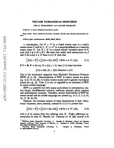
FIG. 1. (Color online) Geometry considered for the variational principle. The wave front ΩF (red) with unit normal vector ~n has passed in all points of the volume V . The interface of V with the domain boundary is a surface ΩD with outward normal vector ~n. Only at the edge C of the wave ~ front, the vector field ~n is discontinuous; there we define N as the outward normal vector to the medium.

on the wave front with determinant h and matrix inverse hAB . In isotropic media, gab is the identity matrix, while in systems with anisotropic diffusion it can be taken equal to the inverse diffusion tensor to capture spatially varying anisotropy [18, 19]. The coordinate change allows writing the linear velocity-curvature relation (5) as: X˙ a = c0 na + γD2 X a ,

(9)

with unit normal to the front AB...F ab...g ng = √ ∂A X a ∂B X b ...∂F X f h(N − 1)!

(10)

where the ... are the fully antisymmetric Levi2 Civita √ −1 symbols. √ AB Furthermore, in Eq. (9), D = ( h) ∂A ( hh ∂B ) is a N − 1 dimensional covariant Laplacian with respect to the tangential coordinates σ A . To prove our theorem (1), (6), we have to show that δV = ~n, ~ δX

δS = K~n ~ δX

(11)

under appropriate boundary conditions. When the wave front touches the domain boundary, the surface bordering the volume where the wave has passed can be divided into the wave front surface ΩF and the surface ΩD where the occupied volume touches the domain boundary. This situation together with the outer normal vectors is sketched in Fig. 1. The N −2 dimensional border between ΩF and ΩD is C, the wave front boundary. In this work, we will not consider broken wave fronts (scroll waves), and assume that wave fronts only end on the domain boundary. In this case, the volume where the wave has passed has a border Ω = ΩF ∪ ΩD ∪ C that is a closed surface. We will assume that the wave front intersects the boundary

3 orthogonally, such that we can impose: ~ || ~n, ∀~x ∈ ΩF : δ X ~ · ~n = 0, ∀~x ∈ ΩD : δ X ~ is continuous across C. ∀~x ∈ C : δ X

delivering Z δS = (12)

The first condition is the transverse gauge, in which we convene without loss of generality that points of the wave front move orthogonally to it. The second condition ensures that the wave front does not propagate across the domain boundary, but allows reparameterization of the interface. The third condition is compatible with the first two only when the wave front ends orthogonally on the domain boundary. This situation automatically follows if the physical boundary is impermeable to the reactants of the underlying system and if the spatial variations in the domain boundary are of length scales bigger than the wave front thickness. In a first step, we construct the volume occupied by the wave front. Take the origin of the Cartesian coordinate system in the region where the front has passed. The volume of the cone with the apex at the origin and an elementary surface area of the wave √ front as the base is ~ · ~ndS with dS = hdN −1 σ, whence dV = (1/N )X I AB...F √ ab..g ∂A X a ∂B X b ...∂F X f X g . (13) V = dS N! h Ω H We have used the symbol to emphasize that the integration runs over the closed surface Ω. Under small ~ A ) in the direction of the wave front norvariations δ X(σ mal only, the resulting change of volume is the functional differential I AB..F ab..g δV = dN −1 σ[∂A δX a ....∂F X f δX g N! Ω + .... + ∂A X a ....∂F δX f X g + ∂A X a ...∂F X f δX g ] I AB..F ab..g dN −1 σ[−δX a ....∂F X f δ∂A X g = N! Ω − .... − ∂A X a ....δX f ∂F X g + ∂A X a ...∂F X f δX g ] I N −1 AB..F ab..g d σ √ ∂A X a ...∂F X f δX g = (N − 1)! Ω h I ~ = dS ~n · δ X. (14) Ω

In the first equality, we performed integration by parts and the boundary terms always vanish due to integration over a closed surface. For the second equality, we renamed a ↔ g in the first term, followed by a transposition in the Levi-Civita symbol, such that the alphabetic ordering of indices is restored. Doing this for the (N-1) first terms yields the desired result. The last line of Eq. ~ = ~n, proving the first statement (14) implies that δV /δ X in Eq. (11). Secondly, we vary the wave front surface Z Z √ S = dS = hdN −1 σ, (15)

ΩF

Z =

Z √ 1 δh dN −1 σ √ = d2 σ hhAB δhAB 2 2 h √ ~ · ∂B δ X ~ dN −1 σ hhAB ∂A X

ΩF

Z =

√ ~ · δX ~ + B.T. dN −1 σ∂B ( hhAB ∂A X)

ΩF

Z =

~ · δ X. ~ dS D2 X

(16)

ΩF

~ = D2 X ~ = K~n if the boundary term Therefore, δS/δ X (B.T.) vanishes. Indeed, using the divergence theorem with respect to coordinates σ A , we find Z √ ~ · δ X) ~ B.T. = dN −1 σ∂B ( hhAB ∂A X (17) ΩF Z I ~ · δ X) ~ = ~ · δX ~ = 0. = dSdiv(gradX d` N ΩF

C

~ is the domain boundary at the wave front edge C. Here, N Then, by Eq. (12), the boundary term vanishes. Hence we have demonstrated that relation (5) can be written as a gradient system. We conclude that in its motion, a non-linear wave front strives to enlarge its occupied volume, while minimizing its surface area. The corollary (2) then states that Z Z 2 2 2 ˙ ˙ γ S −c0 V = −c0 S −γ K dS +2γc0 KdS ≤ 0. (18) which is the analogue of the law for vortex filaments by Biktashev et al. [20]. In particular, for dissipative structures (i.e. when c0 = 0) which are studied in the context of pattern formation, one has that Z S˙ = −γ K 2 dS. (19) Thus, for positive surface tension γ, dissipative structures evolve towards a minimal surface. Discussion. We have shown that the geometric law of motion (5) elegantly follows from an action principle that involves only the simplest geometric invariants of a closed surface. In physics, variational principles have allowed to regard the equations of motion in a more abstract manner, and enabled powerful generalizations. Famous examples include the principles of Fermat and D’Alembert, the Hamiltonian and Lagrangian approach to classical mechanics, and their extensions to quantum theory. Other applications of variational principles are the approximation of eigenstates using the Ritz method and imposing constraints in theoretical and numerical problems of fluid dynamics and continuum mechanics. For non-linear vortices, an extremum principle was found for stationary vortex filaments in [21, 22]. However, a front with non-vanishing plane-wave speed c0 will never reach a final state unless the wave front itself vanishes. Therefore, it should be of no surprise that the

4 variational principle which we identified here is of the gradient rather than the extremum type. At this point, we mention that the terms in the gradient potentials F which we found are highly similar to geometric actions in string theory. Namely, the surface term (15) is identical to the Nambu-Goto string action term, while the volume term (13) has the form of a coupling with an antisymmetric (Kalb-Ramond) field. For propagating dissipation waves, this field happens to be the volume form of the wave front surface [23]. One may wonder whether a similar variational principle will hold for vortex filaments in extended media. Such filaments can be formed after break-up of a traveling wave front due to the velocity-curvature relation (5). A scroll wave filament with arc length parameter s is known to obey the geometric law of motion [18, 20, 24]:

X˙ k /δX i = −2γ2 ∂s3 X j ijm , which does not satisfy the criterion unless γ2 = 0. This condition is fulfilled in chemical systems in which all reactants diffuse at the same rate. Thus, the purely dissipative filament dynamics in such systems with no-flux boundary conditions can be written as a gradient system with potential F = γ1 L,

(21)

If this equation of motion can be written as a gradient system, it needs to satisfy the compatibility condition (4). However, for the law (20), one computes

where L is the total filament length. The corollary (2) recovers the known property that filament length changes monotonically in time [20]. In summary, we have managed to formulate a simple variational principle for the emergent dynamics of propagating non-linear waves in a N-dimensional medium with obstacles. Our result is also a contribution to complexity theory, since we have been able to identify general laws for a wide class of natural systems, without knowing the details of the underlying microscopic processes, and even without knowing the type of partial differential equations that are needed to describe it. Acknowledgements. H.D. was funded by the FWOFlanders.

[1] Y.B. Zeldovich and D.A. Frank-Kamenetsky. A theory of thermal propagation of flame. Acta. Physicochim., 274:341–350, 1938. [2] S. Nettesheim, A. von Oertzen, H.H. Rotermund, and G. Ertl. Reaction diffusion patterns in the catalytic cooxidation on pt(110): Front propagation and spiral waves. J. Chem. Phys., 98:9977–85, 1993. [3] A.M. Zhabotinsky and A.N. Zaikin. Autowave processes in a distributed chemical system. J. Theor. Biol., 40:45– 61, 1973. [4] S. Weinberg. The Quantum Theory of Fields, volume 2. Cambridge University Press, Cambridge, UK, 1995. [5] J. Lechleiter, S. Girard, E. Peraltal, and D. Clapham. Spiral calcium wave propagation and annihilation in Xenopus Laevis oocytes. Science, 252:123–126, 1991. [6] A.L. Hodgkin and A.F. Huxley. A quantitative description of membrane current and its application to conduction and excitation in nerve. J. Physiol., 117:500–544, 1952. [7] R.E. Klabunde. Cardiovascular Physiology Concepts. Lippincott Williams & Wilkins, Baltimore, MD, 2004. [8] O. V. Aslanidi and O. A. Mornev. Can colliding nerve pulses be reflected? Journal of Experimental and Theoretical Physics Letters, 65(7):579–585, 1997. [9] Prigogine I. and Stengers I. Order Out of Chaos. Bantam books, New York, 1984. [10] Morris W. Hirsch, Stephen Smale, Robert L. Devaney, and Morris W. Hirsch. Differential equations, dynamical systems, and an introduction to chaos. Academic Press, San Diego, CA, 2nd ed edition, 2004. [11] O.A. Mornev. Modification of the biot method on the basis of the principle of minimum dissipation (with an application to the problem of nonlinear concentration waves in an autocatalytic medium). Russ J Phys Chem, 72:112–

118, 1998. [12] T. Frankel. The geometry of physics. Cambridge University Press, Cambridge, 1997. [13] O.A. Mornev, A.V. Panfilov, and R.R. Aliev. FitzhughNagumo equations are a gradient system. Biofizika, 37(1):123–125, 1992. [14] E. Yanagida. Mini-maximizers for reaction-diffusion systems with skew-gradient structure. J. Differential Equations, 179:311–335, 2002. [15] J.P. Keener. A geometrical theory for spiral waves in excitable media. Siam J Appl Math, 46:1039–1056, 1986. [16] H. Dierckx, O. Bernus, and H. Verschelde. Accurate eikonal-curvature relation for wave fronts in locally anisotropic reaction-diffusion systems. Phys Rev Lett, 107:108101, 2011. [17] A.V. Panfilov and J.P. Keener. Dynamics of dissipative structures in reaction-diffusion equations. SIAM J. Appl. Math., 55:205–219, 1995. [18] H. Verschelde, H. Dierckx, and O. Bernus. Covariant stringlike dynamics of scroll wave filaments in anisotropic cardiac tissue. Phys. Rev. Lett., 99:168104, 2007. [19] R.J. Young and A.V. Panfilov. Anisotropy of wave propagation in the heart can be modeled by a riemannian electrophysiological metric. Proc Natl Acad Sci USA, 107:15063–8, 2010. [20] V.N. Biktashev, A.V. Holden, and H. Zhang. Tension of organizing filaments of scroll waves. Phil. Trans. R. Soc. Lond. A, 347:611–630, 1994. [21] M. Wellner, O.M. Berenfeld, J. Jalife, and A.M. Pertsov. Minimal principle for rotor filaments. P Natl Acad Sci USA, 99:8015–8018, 2002. [22] K.H.W. ten Tusscher and A.V. Panfilov. Eikonal formulation of the minimal principle for scroll wave filaments. Phys. Rev. Lett., 93:108106, 2004.

~˙ ~ + γ2 ∂s X ~ × ∂s2 X. ~ X(s, t) = γ1 ∂s2 X

(20)

5 [23] B. Zwiebach. A first course in string theory. Cambridge University Press, Cambridge, 2004.

[24] J.P. Keener. The dynamics of three-dimensional scroll waves in excitable media. Physica D, 31:269–276, 1988.