EDUCATION
Revista Mexicana de F´ısica E 59 (2013) 56–64
JANUARY–JUNE 2013
Variational approximation for wave propagation in continuum and discrete media L. A. Cisneros-Ake Departmento de Matem´aticas, Escuela Superior de F´ısica y Matem´aticas, Instituto Polit´ecnico Nacional, Unidad Profesional Adolfo L´opez Mateos Edificio 9, M´exico 07738 D.F., M´exico. e-mail:
[email protected]. Received 27 August 2012; accepted 16 April 2013 We develop a variational approximation for wave propagation in continuum and discrete media based on the modulation of wave profiles described by appropriate trial functions. We illustrate the method by considering an application to the theory of dislocation of materials. We first consider the continuum approximation of the model and reproduce the exact traveling known solution. We then consider the fully discrete non integrable model and obtain an approximate solution based on trial functions with functional form similar to the exact solution of the continuum. The description of this discrete approximate solution is in terms of a discrete nonlinear dispersion relation between the wave parameters. In this last situation we compare the numerical and variational solutions at the stationary case. We thus illustrate the usage of a variational asymptotic approximation to study nonlinear problems and we contrast the differences and difficulties between continuum and discrete problems. Keywords: Modulation theory; average Lagrangian; trial function. PACS: 62.20.mm; 63.20.Pw.
1.
Introduction
According to classical mechanics the description of physical variables, which describe a given physical problem, are well defined at each instant of time. Actually, the temporal evolution of a physical system is completely determined if its state is known at a given initial time [1]. Mathematically this fact is expressed by a set of ordinary or partial differential equations (equations of motion) subjected to certain provided initial and/or boundary conditions. The classical idea is to consider the physical variables involved and to formulate temporal equations of motion to predict its temporal evolution. A typical way to obtain classical mechanics systems is by using Newton’s laws. In particular, the second law of Newton provides a second order ordinary differential equation for the temporal evolution of position of a mass subjected to an external force. A variety of examples in classical dynamical systems in one independent variable (the position of the object) is given by mass-spring dynamical systems. In case of several independent physical variables Newton’s laws produce equations of motions described by partial differential equations, an example of this fact is given by the string’s equation which corresponds to the wave, in general, nonlinear equation. Numerical and asymptotic approximations are usually used to study the behavior of the solutions for the equations of motion expressed, in general, by nonlinear differential equations. A different approach to obtain the equation of motion for a physical system is by means of variational principles. This method is based on the idea that the physical system has to evolve through the trajectory of “minimal resistance” [2]. Historical examples based on this minimal principle are the problem of the minimal trajectory of a reflected ray in a different medium, the Fermat’s principle which establishes that
incident rays travel following the trajectory of shortest time, and the brachistochrone or cycloid problem corresponding to the curve for the shortest descending time of a point mass. These problems were initially studied by algebraic means and primitive (first) ideas of differential calculus. It was until the end of the XVIII century when Leonard Euler (1701-1783) and Joseph Louis Lagrange (1736-1813) set down the bases of the modern calculus of variations that the optimization of variable functions, called functionals, on an admissible set of solutions was possible in a more systematic way. The basic idea of variational calculus is that the functional (called the Lagrangian of the system) associated to the equation of motion, via the inverse problem of the calculus of variations, has an extreme value at the solution of the dynamical system. This extreme value is obtained when the so called Euler-Lagrange equations of the associated variational problem are satisfied [3,4]. Variational principles were first explicitly used to study the propagation of water waves by Luke in 1967 [5]. The variational approximation in the context of wave phenomena modulates amplitude and frequency, which for the nonlinear case are related between each other by nonlinear dispersion relations, of the propagating waves in order to extremize the corresponding Lagrangian of the system. In this paper we develop the modulation theory of Whitham [6], which is based on the extremization of the functional associated to the given equation of motion, for continuum and discrete systems. This functional is given, via the inverse problem, by the averaging in the independent variables of the physical problem of the Lagrangian for the equations of motion of the system. The extremization in the modulation theory is in terms of a set of wave parameters generating a family of solutions (admissible set of solutions), called trial functions or anzats. Thus the Euler-Lagrange equations
VARIATIONAL APPROXIMATION FOR WAVE PROPAGATION IN CONTINUUM AND DISCRETE MEDIA
for the parameters generated by the proposed trial functions will provide in general nonlinear coupled ordinary differential equations whose solutions, joint with the proposed trial function, will correspond to the extreme (minimum) of the Lagrangian for the solution of the equations of motion [6]. That is, in the functional space generated by the trial functions we will variationally get the nearest asymptotic solution to the “exact” one for the given equations of motion. This variational approach has been employed in several works in different contexts both in the continuum and discrete cases, see for example [7-11]. We illustrate how the modulation theory works in continuous and discrete problems by considering an application to the theory of dislocation of materials for the propagation of fractures [12-14]. The equations of motion are based on a double well potential given by the φ4 model [15].
2. Variational formulation A functional is a rule that assigns a real number to each function y (x) on a well defined class of functions A, called admissible set of functions, which can be for example the set of continuous functions in the interval [a, b] or the set of continuously differentiable functions in [a, b] satisfying y (a) = y (b) = 0. In most of the applications the functionals are expressed as Zb J (y) = L (x, y, y 0 ) dx a
with y ∈ A. The integrand L = L (x, y, y 0 ) is called the Lagrangian of the equation of motion describing the application, since it coincides with the Lagrangian of classical mechanics [2]. Similar to calculus in real variables we require to find the extreme values of the functional in order to optimize it. The fundamental theorem that provides the extreme values states that if y is an extreme for the functional
therefore the Euler-Lagrange Eq. (1) is in general a second order nonlinear ordinary differential equation for y thus reminding, in some sense, Newton’s second law of motion. The inverse problem of calculus of variation establishes that a physical system has a variational principle if there is a Lagrangian L for the equations of motion such that the EulerLagrange equations for the action integral Zt2 Z Ldxdt,
L= t1 R
called the average Lagrangian, reproduce the equations of motion for the physical system [4]. For mechanical systems L = T − V where T and V are the energy densities. We thus can formulate a physical problem, expressed by equations of motion, into a variational formulation by comparing and integrating the differential Eq. (2) with the given equations of motion to get the appropriate Lagrangian L for the system. The inverse problem of calculus of variation for time dependent continuum and discrete problems in one space dimension typically provides Lagrangians in the form:
and
L = L (t, u, ux , ut ) ,
(3)
³ · ´ L = L t, un , un−1 , un , un+1 ,
(4)
·
respectively. Where un = (d/dt)un and u = u (x, t), un = un (t) are assumed to satisfy the given continuum or discrete equations of motion. We now consider the average Lagrangian for the continuum and discrete cases in the form: Zt2 L=
Z dt
t1
L=
dt t1
L (x, y, y 0 ) dx
L (t, u, ux , ut ) dx,
(5)
R⊂R
Zt2
Zb J (y) =
57
X
³ · ´ L t, un , un−1 , un , un+1 ,
(6)
n∈R⊂Z
where y (a) = y1 , y (b) = y2 then y satisfies the ordinary differential equation
where R is the appropriate spatial region where the object under study is allowed to move. We thus can come back to the corresponding equations of motion by considering the total variation δL = 0 of the functionals (5) and (6)
∂ d ∂ L− L = 0, 0 dx ∂y ∂y
∂ ∂L ∂L d ∂L + − = 0, dt ∂ut ∂x ∂ux ∂u
(7)
∂L d ∂L − = 0. dt ∂ u· n ∂un
(8)
a
(1)
which is known as the Euler-Lagrange equation. It is remarked that the Euler-Lagrange Eq. (1) is obtained when the total variation of the function equals zero, that is δJ = 0, and is the variational analog of the condition in the derivative for critical points in differential calculus [3]. The chain rule applied to the previous Eq. (1) gives Ly0 x + Ly0 y y 0 + Ly0 y0 y 00 − Ly = 0,
(2)
and
In the modulation theory of Whitham [6] we must assume that the equation (continuum or discrete) of motion posses a family of solutions, called trial functions or anzats, depending on a coherent vector of slowly varying parameters
Rev. Mex. Fis. E 59 (2013) 56–64
58
L. A. CISNEROS-AKE
a = a (t) in the form u = U (x − ξ (t) , t, a) for the continuum and un = U (n − ξ (t) , t, a) for the discrete problem · respectively, where da/dt = a ¿ 1. The modulation theory developed by Whitham reduces to the well known collective variables approach when the coupling between the coherent structure and its linear shedding radiation is neglected. This collective variables approach gives at first order the same results as the modulation theory and it has been used widely by different authors in different applications (see the book of O. M. Braun and Y. S. Kivshar [16]). However in some cases is important to considerer higher order approximations in order to get the appropriate interaction between the wave parameters of the trial function. In most of the situations the linear radiation in the modulation theory provides a damping term in the equations for the wave parameters [17-19]. We thus substitute the trial functions u = U (x − ξ (t) , t, a) and un = U (n − ξ (t) , t, a) into the corresponding average Lagrangian (5) and (6) to obtain Zt2 L=
¶ Z∞ µ dt L t, U (x, t, a) , Ux (x, t, a) , Ut (x, t, a) dx
t1
−∞
Zt2
µ
=
F
substitution of un = U (n − ξ(t), t, a) in (11) and from the Poisson summation formula [20] ∞ ³ · ´ X L t, un , un−1 , un , un+1 n=−∞
=
b is the Fourier transform of where G ·
L=
dt t1
³ · ´ L t, un , un−1 , un , un+1
∞ X n=−∞
Zt2 X ∞
2πimξ
e
µ ¶ · · b G m, a, ξ, a dt,
(10)
t1 m=−∞
respectively. The functional term ¶ Z∞ t, ξ, a = L (t, U (x, t, a) , Ux (x, t, a)) dx ·
−∞
provides the spatial averaging of the Lagrangian L in the continuum. For discrete problems a typical Lagrangian takes the form: ³ · ´ L = L t, un , un−1 , un , un+1 = T − V =
·
in the variable z = n − ξ(t). We must note that the last expression (12) has periodic terms for m 6= 0 due to the factor e2πimξ that comes from the shifted site n − ξ(t) in the Poisson’s formula. These periodic terms correspond to an internal periodic potential generated for the lattice equations of motion itself and are known as the Peierls-Nabarro (PN) potential. We thus remark that this PN potential characterizes lattice problems in contrast to the continuous ones. Also, in the limit when the amplitude of the PN terms, called the PN potential barrier, go to zero we recover the limit of the continuum media. We now consider the higher modes of (12) to get, for the average Lagrangian (12) to second order approximation in ·
·
the Poisson formula, a quadratic form in ξ and a:
(9)
and
F
·
G = G(n − ξ(t), a, ξ, a) = L(t, un , un−1 , un , un+1 )
·
Zt2
(12)
m=−∞
· ·
·
b (a) , + C (a, ξ) a2 + exp (2πiξ) G
t1
µ
µ ¶ · b m, a, ξ, a· , e2πimξ G
L = A (a, ξ) ξ 2 + B (a, ξ) ξ a
¶ · t, ξ, a dt,
=
∞ X
1 ·2 1 2 u − (un+1 − un ) − V (un ) , 2 n 2 2
(11)
where the terms (1/2) (un+1 − un ) and V (un ) correspond to on-site and substrate interactions, respectively. Thus after
(13)
where the coefficients A (a, ξ), B (a, ξ) and C (a, ξ) are those arising in the Poisson summation expansion of (12) to second order. We thus obtain for the full discrete system a Lagrangian for a particle whose position ξ (t) is moving in an external periodic potential, exp (2πiξ), created by the lattice itself with internal degrees of freedom described by a vector of parameters a. We remark that in the continuum limit the b (a) vanishes and a typical averperiodic term exp (2πiξ) G age Lagrangian, as the given by (9), is recovered. In the modulation theory of Whitham after the averaging of the Lagrangian we must take the total variation δL = 0 of the Lagrangians (9) and (10) to obtain ordinary differential equations for the parameters describing the trial function. These ordinary differential equations correspond to the EulerLagrange equations for the parameters ξ and a in the trial function. In general however there will be linear radiation losses due to non integrability of the equations of motion or due to non suitable trial functions. Figure 1 shows a typical leading wave profile shedding linear radiation in a continuum medium that comes from solving the Korteweg-de Vries (KdV) equation ut + 6uux + uxxx = 0 for nonsoliton initial conditions [17]. The initial condition in this case evolves to an exact coherent soliton solution in the completely integrable KdV by shedding linear radiation.
Rev. Mex. Fis. E 59 (2013) 56–64
VARIATIONAL APPROXIMATION FOR WAVE PROPAGATION IN CONTINUUM AND DISCRETE MEDIA
59
solutions in continuum and discrete media. In order to do this with maneageble computations we consider the continuous and discrete φ4 model in the theory of dislocation materials and approximate traveling kink solutions. In the approximation we do not consider the linear shed radiation in order to illustrate the computations and because in practice the linear radiated waves represent small damping terms in the EulerLagrange equations for the parameters in the trial functions.
3.
F IGURE 1. Typical leading wave profile shedding linear radiation in a continuum medium.
The radiation losses should be included using conservation laws to balance the conserved quantities due to the interaction between the solutions and the linear radiation dispersed. We thus have to include the shed radiation to obtain equations for the parameters in a closed form. The general idea to do this is to consider a conserved quantity by the Lagrangian, for example, the total energy ·
·
·
function E(u, u) and the average energy E(ξ, a, ξ, a) we then use the conservation law for the Lagrangian: ³ ·´ ³ ·´ d d ³ ·´ d E u, u = Ec u, u + Er u, u , (14) dt dt dt where Ec is the energy of the leading wave or coherent structure and Er is the energy taken by the dispersed radiation at the tail of the leading wave (see Fig. 1 for example). We now
Edge dislocation dynamics
Some mechanical properties of solids are modeled by differential-difference equations. Pioneering works by [12-14] on dislocations in metals established the well known Frenkel-Kontorova model as the governing equation. The Frenkel-Kontorova was the first model to explain in simple terms the edge dislocation dynamics in a material at atomic level. The main idea behind this model is to consider a semi-infinite plane of atoms inserted from one side to the next due to a lateral force applied to a perfect rectangular crystal lattice. After the systems relax to an equilibrium state a lateral dislocation in the crystal lattice takes place. A layer of atoms perpendicular to the inserted plane due to the dislocation divides the crystal into two different parts, see Fig. 2. The atoms in the interface layer are subjected to an external substrate periodic potential, generated by the surrounding atoms in the upper and lower layers of the crystal lattice, that is well approximated in the form: φs =
E0 (1 − cos (α0 yn )) , 2d2
(15)
where E0 /2d2 is the distance between the interface layer and its the upper and lower layers, α0 /π is the transversal distance between neighboring atoms and yn denotes the relative displacement of the nth atom with respect to its neighboring atoms along the interface layer.
corresponding to the flux energy transferred between the coherent structure and the linear radiation. To close the equations we just need to compute F . For mechanical systems F is given by a quadratic form (when a small radiation is assumed) corresponding to an absorbed or dissipated potential at the boundary between the coherent structure and the radiation. To compute F we need to know the value of the radiation at the boundary and then to solve the equations of motion for the shed waves. The boundary value is determined using global balances of energy and a detail coupling between the coherent structure and the radiation [21]. In principle it is always possible to develop the last analysis for the variational approach. However it is a difficult matter to find appropriate trial functions and to solve the linear equations for the radiated terms because the leading profile should be coupled to the radiated wave in moving domains, see Fig. 1. In the following sections we illustrate how the modulation theory approach works to approximate traveling wave
F IGURE 2. Cross section at the molecular level of a 3D edge dislocated material with a rectangular crystal structure.
·
·
·
use that Ec (u, u) = E(ξ, a, ξ, a) and the quantity ³ ·´ d F = Er u, u , dt
Rev. Mex. Fis. E 59 (2013) 56–64
60
L. A. CISNEROS-AKE
Since the crystal lattice is rectangular in shape and due to the external periodic potential produced by the neighboring atoms, the dynamical equation for the atoms in the interface layer (which actually represents the fracture in the material) obeys the Frenkel-Kontorova (FK) model: E0 α0 sin (α0 yn ) , my n =C (yn−1 −2yn +yn+1 ) − 2d2 ··
(16)
where the term yn−1 − 2yn + yn+1 is obtained from the nearest neighbor interaction in the rectangular crystal lattice, m denotes the same mass in all the atoms and C is the coupling factor (shown as springs in Fig. 2) between neighboring atoms. The FK model supports kink solutions interacting strongly with radiation losses [9,22]. For relatively small displacements of the dislocation, the external periodic potential φs in the FK model is well approximated by the double well bi-stable φ4 potential: φr = −(A/2d2 )yn2 + (B/4d2 )yn4 for appropriate fit parameterspA and B in the form E0 = −(A2 /4B) and α0 = π B/A, see Fig. 3. In order to get a better understanding of the computations in the modulation theory, instead of the periodic potential φs in the FK model we consider the double well potential given by the φ4 model: ¢ 1 ¡ Ayn −Byn3 . (17) 2 d p We now consider the change of variables yn0 = yn B/A, p t0 = t A/m and C 0 = C/A to obtain the non dimensional system: ··
my n =C (yn−1 −2yn +yn+1 ) +
··
y n = C (yn−1 − 2yn + yn+1 ) +
¢ 1 ¡ yn − yn3 , 2 d
(18)
where the primes have been removed for simplification. In the limit d → ∞ and for C = 1 we recover the well known φ4 continuum equation model utt = uxx + u − u3 .
(19)
This last equation has exact traveling kink solutions. We check this fact by considering u = u (x, t) = f (x − vt) and f → σ = ±1 when |z| = |x − vt| → ∞. We substitute these conditions into Eq. (19) to obtain: ¢ d2 f 1 ¡ = 2 f − f3 . 2 dz v −1 We then separate variables to get: µ ¶ 1 f4 f 02 = 2 f2 − + A. v −1 2 f 00 =
(20)
(21)
The condition at infinity on f (z) gives A = 1/2(1−v 2 ). Again separation of variables produces: Zf 0
dw = 2 |w − 1|
Zz x0
ds √ √ . 2 1 − v2
(22)
Integration of last expression gives the traveling kink solution µ ¶ x − vt − x0 u (x, t) = σ tanh √ √ , (23) 2 1 − v2 where σ = ±1 is the kink polarity and 0 ≤ v < 1 the kink velocity. We reproduce in the next section the exact kink solution (23) by means of the modulational approximation in the continuum model (19). 3.1. Modulation theory for the continuum model We may see that the equation of motion (19) is obtained from the Lagrangian ¸ Z∞ · ¢2 1 2 1 2 1¡ 2 L= ut − ux − u −1 dx, (24) 2 2 4 −∞
when the Euler-Lagrange equation d ∂L ∂ ∂L ∂L = 0, + − dt ∂ut ∂x ∂ux ∂u
(25)
is satisfied. We now reproduce the exact kink solution found in the last section by using the modulation theory explained above. To this end we consider the family of trial functions µ ¶ x − ξ (t) u (x, t) = σ tanh , (26) w (t)
F IGURE 3. External substrate interaction potentials. Dashed dot curve: Periodic potential φs = (E0 /2d2 ) (1 − cos (α0 y)). Continuum curve: Double well φ4 potential φr = −(A/2d2 )y 2 + (B/4d2p )y 4 . For A = B = d = 1, E0 = −(A2 /4B) and α0 = π (B/A).
generated by free variable parameters in position ξ (t) and width w (t). The idea is to modulate the variation of these free parameters to recover the exact kink solution (23). We substitute (26) into the average Lagrangian (24) to obtain: L=
Rev. Mex. Fis. E 59 (2013) 56–64
2 ·2 π 2 − 6 ·2 2 w ξ − w − − . 3w 18w 3w 3
(27)
VARIATIONAL APPROXIMATION FOR WAVE PROPAGATION IN CONTINUUM AND DISCRETE MEDIA
We then take variations in the free parameters and find their Euler-Lagrange equations: ·
4 d ξ δξ : = 0, 3 dt w ¡ ¢ ·· 6 · δw : − π 2 − 6 w + ξ 2 w
(28)
π2 − 6 ·2 6 w − + 3w = 0, (29) 2w w where the symbol δ indicates variation. We may notice that Eq. (29) is a nonlinear second order ODE in w. We actually have a stable critical point in δw at: r ·2 √ w = 2 1−ξ , (30) +
61
We finally explain in the next section the modulation theory for the discrete case and observe the new behavior of the modulational solution due to the PN potential. It is to be remarked that the full discrete problem is not completely integrable so that no exact solution is available. This is actually another advantage of using the modulation theory. 3.2.
Modulation theory for the discrete model
The discrete lattice system (17) can be variationally obtained from the average Lagrangian L=
∞ X ¢2 1 ·2 1 1 ¡ 2 yn − (yn − yn−1 ) − 2 yn2 − 1 , (32) 2 2 4d n=−∞
·
for fixed velocity ξ since the linearization of (29) in w shows a center for it. It can be shown numerically [15] that for initial conditions close to (23) the equation of motion (19) radiates linear waves to adjust the initial condition to the exact traveling kink. This fact is reflected in Eq. (29) as an exponential damping term in w [22]. Thus the temporal evolution for w is actually a spiral towards the critical point (30). In this way the exact traveling kink solution is recovered at the critical point of the modulation Eqs. (28) and (29). The Eq. (28) is now integrated twice to find ξ = vt + x0 ,
(31)
·
where v = ξ (0) and x0 = ξ (0) are the initial velocity and position of the kink, respectively. Equations (30), (31) and the anzats (26) recover the exact solution (23).
1 L= 2w2
µ
· 2
w2 ξ − 2 2d
µ
¶ X ∞
4
sech n=−∞
n−ξ w
when the Euler-Lagrange equations d ∂L ∂L − = 0, dt ∂ y· ∂yn
(33)
n
are satisfied. Similar to the previous continuous case we develop our modulation theory by considering as trial function the one suggested by the exact kink solution from the continuum model, that is µ ¶ n − ξ (t) yn (t) = σ tanh . (34) w (t) We then substitute (34) into the average Lagrangian (32) to obtain:
·
µ ¶ ∞ w2 X n−ξ 2 4 + (n − ξ) sech 2w4 n=−∞ w
µ ¶ µ ¶ µ ¶ · ∞ ∞ X ξw X n−ξ n−ξ 1 4 2 + 3 (n − ξ) sech + sech − 2 coth . w n=−∞ w w w n=−∞ ·
(35)
We may notice that the leading term contribution of ∞ X
µ (n − ξ) sech4
n=−∞
n−ξ w
¶ ,
· ·
corresponding to its integral, is zero. We thus neglect the ξ w term. We now use the Poisson summation formula to find the second order approximation of the infinite series in the average Lagrangian ¶ µ· · w2 2 (36) L = ξ − 2 f1 (w, ξ) + w2 f2 (w, ξ) + f3 (w, ξ) , 2d where
¡ ¢ µ ¶ ∞ 4π 2 1 + π 2 w2 1 X n−ξ 2 4 f (w, ξ) = sech ≈ + cos (2πξ) , 2w2 n=−∞ w 3w 3 sinh (π 2 w) 1
Rev. Mex. Fis. E 59 (2013) 56–64
(37)
62
L. A. CISNEROS-AKE
µ ¶ ∞ 1 X n−ξ π2 − 6 2 4 f (w, ξ) = (n − ξ) sech ≈ 2w4 n=−∞ w 18w " ¡ ¢ ¡ ¢ ¡ ¢ # 3 π 2 − 2 + π 4 w2 + π 2 + 6 + π 4 w2 cosh 2π 2 w π 2 cos (2πξ) − , ¡ ¢ ¡ ¢ 6 sinh3 (π 2 w) −2 w1 + 3π 2 w sinh 2π 2 w µ ¶ µ ¶ ∞ X 1 n−ξ 2 3 f (w, ξ) = sech − 2 coth ≈ 2w w w n=−∞ µ ¶ 1 4π 2 w2 − 2 coth + cos (2πξ) . w sinh (π 2 w) 2
(38)
(39)
We take variations of the discrete kink’s parameters and write down their Euler-Lagrange equations ·µ · ¶ ¸ · ·· · · 1 w2 ∂ξ : ξ = − 1 ξ 2 + 2 fξ1 + 2ξ wfw1 − w2 fξ2 − fξ3 , 2f 2d · µ· ¶ ¸ · · · 1 w 1 w2 ·· 2 1 2 2 2 3 ∂w : w = − 2 f − ξ − 2 fw + 2ξ wfξ + w fw − fw , 2f d2 2d
(40) (41)
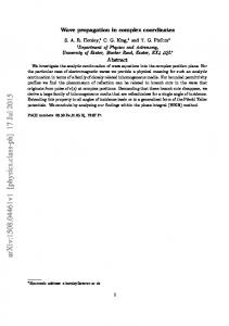
where the subindex indicates partial derivative with respect to that variable of the indicated function. We notice that similar to the continuum case the extreme of the average Lagrange (32) is reached at the critical point of (41) given by µ· ¶ w 1 w2 2 f − ξ − fw1 − fw3 = 0. (42) d2 2d2 We thus simplify the last expression using (37)-(39) to obtain at first order in the Poisson summation formula the discrete nonlinear dispersion relation à ! · 6d2 w2 2 2 ¡ ¢ . (43) ξ = 2 −1 + 6d − 2 2d w sinh2 w1 For large w last expression recovers the dispersion relation of the continuum model F IGURE 5. Comparison in the core region between the modulation ·
theory and the numerical solution in the stationary state ξ = v = 0 at ξ = 0 for d = 0.9 and C = A = B = 1. a) Numerical difference between the numerical and modulation solutions, b) graphs of the numerical and modulation solutions.. ·
ξ2 = 1 −
F IGURE 4. Continuum curve: Dispersion relation (43) for the discrete case. Dashed curve: Dispersion relation (44) for the continuous case. In both cases d = 0.9.
w2 . 2d2
(44)
Figure 4 shows the comparison between the discrete dispersion relation (43) and the continuous one (44). We finally consider the modulation approximation obtained from the kink profile (34) and wave parameters according to the nonlinear discrete dispersion relation (43) and compare it with the exact kink solution in the discrete case obtained by numerical means. To this end we consider the ·
stationary state ξ = v = 0 at ξ = 0 for the discrete system (18) in the form:
Rev. Mex. Fis. E 59 (2013) 56–64
VARIATIONAL APPROXIMATION FOR WAVE PROPAGATION IN CONTINUUM AND DISCRETE MEDIA
0 = C (yn−1 − 2yn + yn+1 ) ¢ 1 ¡ Ayn − Byn3 = f (..., yn−1 , yn , yn+1 , ....) . (45) 2 d We proceed in this way since in our modulation analysis we neglected the PN effects and considered the steady state
for the wave parameters. We now solve (45) numerically by using Newton’s method as follows:
+
Ak = Jf (Y) |Y=Yk
. . . . . .
¡ k¢ Yk+1 = Yk − A−1 , k f Y
−2C +
is the jacobian of the function f at the kth iterate. We then consider (34) as an initial iterate for Newton’s method (46) to obtain the full numerical solution at the steady state. Figure 5a) shows the difference in the core region between the numerical solution ynnum obtained from Newton’s method and the modulation solution ynmod obtained from the trial function (34) and the dispersion relation (43) at d = 0.9. Figure 5b) corresponds to the profiles ynnum and ynmod . We observe a remarkable comparison. We thus have shown how the variational approximation produces solutions to nonintegrable discrete models. The discrete φ4 model as presented here is not reported in the literature and illustrates how to proceed in discrete media.
4. Conclusions We developed the modulation theory in continuum and discrete systems. In the case of the φ4 model, for edge dislocations in materials, its discrete version is not integrable and no analytical solution is available. We reproduced the exact kink solution of the continuum model and showed in the discrete case that the variational approximation provides an extreme solution for a kink profile similar to the exact solution of the continuum counterpart. The nonlinear dispersion relation obtained for the discrete case is not reported in the literature and
(46)
¢ ¡ k k , ynk , yn+1 , ... is the kth iterate and where Yk = ..., yn−1
. . .
= . . C . . . . . . . . .
63
1 d2
. . ³ . ¡ ¢2 ´ A − 3B ynk . . .
. . . C . . .
. . .
. . .
. . , . . . . . .
(47)
explains the qualitative effects of the discreteness. Thus the modulation theory gives a quasi-analytical description of the solution which presents a remarkable comparison with the full numerical solution of the problem at the steady state obtained from Newton’s method. The variational ideas presented in this work can be used in other continuum or discrete nonintegrable problems where there is no exact solution. For instance, the Galilean problem of a hanging chain which has a cosine hyperbolic solution in the continuum. In the discrete version of this problem a similar phenomenon in the solution as the one described here can be found. We finally remark that this work can be helpful to people interested in approximate solutions to nonlinear problems in discrete and continuum media. This work is also developed to introduce to students to more advanced papers that use variational approaches to get approximate solutions.
Acknowledgments The author thanks the financial support from COFAA-IPN, IPN-CGPI-20130803 and Conacyt project 177246. Thanks are also expressed to the anonymous referees for their useful comments, which substantially improved this work, and to professor Tim Minzoni for helpful discussions.
1. G. R. Fowles and G. L. Cassiday, Analytical Mechanics (Brooks Cole, Seventh Edition, 2004).
6. G. B. Whitham, Linear and Nonlinear Waves. (A WileyInterscience series of texts, monographs and tracts, 1999).
2. H. Goldstein, C. Poole and J. Safko, Classical Mechanics (Addison Wesley, Third Edition, 2000).
7. M. Syafwan, H. Susanto, S. M. Cox and B. A. Malomed, J. Phys. A: Math. Theor. 45 (2012) 075207.
3. I.M. Gelfand and S.V. Fomin, Calculus of Variations (PrenticeHall, Englewood Cliffs, NJ, 1963).
8. H. Susanto and P. C. Matthews, Phys. Rev E, (2011) 035201.
4. Lokenath Debnath, Nonlinear partial differential equations for scientists and engineers (Birkhauser Boston, 1997). 5. J. C. Luke, J. Fluid Mech. 27 (1967) 395.
9. L. A. Cisneros and A. A. Minzoni, Physica D 237 (2008) 50. 10. L. A. Cisneros and A. A. Minzoni, Studies in Applied Mathematics 120 (2008) 333.
Rev. Mex. Fis. E 59 (2013) 56–64
64
L. A. CISNEROS-AKE
11. A. B. Aceves, L. A. Cisneros-Ake and A. A. Minzoni, Discrete and Continuous Dynamical Systems - Series S. 4 (2011) 975994. 12. Ya. Frenkel, T. Kontorova: Phys. Z. Sowietunion 13 (1938) 1. 13. T. A. Kontorova, Ya. I. Frenkel: Zh. Eksp. Teor. Fiz. 8 (1938) 89. 14. W. Atkinson and N. Cabrera, Phys. Rev. 138 (1965) A763. 15. J. Andrew Combs and Sidney Yip, Phys. Rev. B 28 (1983) 6873. 16. O. M. Braun and Y. S. Kivshar, The Frenkel-Kontorova model: Concepts, method and applications (Springer-Verlag, 2004).
17. W. L. kath and N. F. Smyth, Phys. Rev. E 51 (1995) 661. 18. W. L. Kath and N. F. Smyth, Phys. Rev. E 51 (1995) 1484. 19. N. F. Smyth and A. L. Worthy, Phys. Rev. E 60 (1999) 2330. 20. L. Debnath and D. Bhatta. Integral transforms and their application, (Chapman & Hall/CRC. 2nd edition2007). 21. A.A. Minzoni, Bol. Soc. Mat. Mex. 3 (1997) 1-49. 22. M. Peyrard and M. Kruskal, Physica 14D (1984) 88.
Rev. Mex. Fis. E 59 (2013) 56–64