Vehicle positioning by database comparison using the ... - CiteSeerX

Vehicle positioning by database comparison using the Box-Cox metric and Kalman filtering Trond Nypan

Kenneth Gade

Oddvar Hallingstad

UniK - Center for Tech. at Kjeller [email protected]

Norwegian Defence Research Establishment [email protected]

UniK – Center for Tech. at Kjeller [email protected]

Abstract-The most accurate mobile station (MS) positioning of today is done using techniques based on time-of-arrival measurements like network assisted GPS and OTDOA. In this paper we present a system for MS positioning based on database comparison of measured location sensitive parameters. We have utilised the estimated channel impulse response (CIR) for comparison. The Box-Cox metric and Kalman filtering is used to yield position estimates along measured streets in a city. System tests are performed using about 30 km of channel sounder measurement data. The positioning system is generic and may thus be developed to include more location sensitive measurement data at a later stage. The results indicate satisfactory positioning in most cases. I.

INTRODUCTION

Location of mobile stations (MSs) has received a lot of attention. It is commonly believed that a great number of new value-added services can be realised using location technology. The proposed applications are many, with functions ranging from traffic navigation, route finding, fleet management, localised news, weather and advertisements. The United States’ Federal Communications Commission decision to mandate location-processing capabilities for Emergency-911 calls increased development in this area substantially [1]. The US network operators are now concentrating on two main technologies. One is based on Global Positioning System (GPS) pseudorange measurements, and the other is based on propagation time measurements between the MS and the base station (BS). The methods developed are now commonly referred to as network assisted GPS (A-GPS) [2] and observed time difference of arrival (OTDOA)1 [3]. For an overview and comparison of these methods, see [4]. Other location methods are based on network available information like cell-id, cell-sector, timing-advanced and received-signal-strength [5]. Hybrid methods using different selections of these parameters often referred to as enhanced cell-id methods, have also been investigated. Some of these methods are operational, yielding value-added services to network operators despite their relatively poor accuracy. T.N. would like to thank Siemens AS and Telenor Mobil AS for sponsoring this research performed at Center for Tech. at Kjeller. 1 The terms time difference of arrival (TDOA) and enhanced observed time difference (E-OTD) are also used for the OTDOA method.

The main disadvantage of A-GPS and OTDOA systems are that they assume line-of-sight (LOS) propagation between the transmitter and the receiver. In general this assumption is not valid in city centres where LOS often is blocked by high-rise buildings. The accuracy of these systems is significantly degraded by the multipath propagation caused by signals bouncing off buildings or other elevated topological features. In mountainous areas characterised by narrow valleys and few base stations both A-GPS and OTDOA performance may degrade severely. In valleys where parts of the sky are blocked, GPS signals are obstructed yielding problems for the positioning process [6]. The OTDOA method requires signalling with three or more base stations and this is rarely the case in such areas. Consequently developers have started to look into other methods of providing location capabilities in multipath areas and particularly in so-called dense urban environments. Database comparison (also referred to as location fingerprinting) techniques have received more attention among developers lately in order to address some of the problems related to non-LOS and multipath propagation [5]. The main idea of the database comparison technique is to map location sensitive parameters of measured radio signals along streets of interest. A database is established and a moving MS can compare its measurements with the ones in the database. In this way the location of a mobile can be estimated. In [7] the parameters used for comparison is the received signal strength as measured by the MS from several nearby BSs. We introduce a new method using the channel impulse response (CIR) for location purposes. The CIR is estimated both by the MS and the BS and used in the demodulation process in wideband communication systems like GSM, UMTS and Digital Audio Broadcasting. Hence no new hardware is required in the MS or at the BS except for a location server containing the database. II.

PHYSICAL BACKGROUND

In build-up and mountainous areas there is most of the time a non-LOS path between the transmitter and the receiver. The main propagation mechanisms are therefore by scattering from the surface of obstacles and diffraction around them. In practise energy arrives via several paths and a multipath situation is said to exist. When measured by a wideband

receiver, the CIR yields an estimate of the number of multiple propagation paths as well as their relative delay and strength. A set of successively measured CIRs, h(t ,τ ) , is depicted in Fig. 1.

Multipath environment

GSM/ UMTS

Base station

Mobile station

40

|h(t,τ)| [dB]

30 20

Location database • Mapped CIRs • Digital maps

10 0 −10 12

−20 0

Fig. 2. Possible architecture of the proposed location system

10 5

8

10

6

15

4

20

IV.

2

25 30

0

Time, t [ms]

Delay,τ [µs]

Fig. 1. Measured set of channel impulse responses

The resolution of the measured CIR depends on the system bandwidth. The effect of a limited bandwidth (see section IV.A) is that multiple reflections may end up in the same time bin on the CIR delay axis. When this occurs, the reflections combine vectorially to yield a resultant signal large or small depending on the distribution of phases among the component waves. When a MS moves the result is a fluctuating signal amplitude. This effect is known as fading, see [8] chapter 14. The delay difference between the CIR maximums corresponds to the distance difference between reflecting surfaces in the channel. When moving towards or from a strong reflector, the corresponding maximum moves to the left or right on the delay axis. This should make the measured CIR a good candidate for database comparison, but fading complicates things due to the random fluctuations of the CIR maximums. The objectives of our pattern recognition algorithm are thus to extract location dependent features of the CIR measurements, and to reduce the influence of fading. III.

DATABASE COMPARISON

The solution space in database comparison is limited to roads already mapped by measurement equipment. A possible architecture of the proposed location system may look like Fig. 2. Measurements using a channel sounder have been collected along streets in typical urban and suburban environments of Münich in Germany. Several measurement runs were performed along the same streets. Later, the various measurement series have been compared using the pattern recognition algorithm described in section IV.

PATTERN RECOGNITION

The pattern recognition algorithm used to process the measurements has the following steps: data acquisition, feature extraction, pre-processing, Box-Cox metric calculation, cost-function calculation, search and decide. The structure of the processing steps is depicted in Fig. 3 and the details are described below. H

h(k)

abs

h1(k)

avg

h2(l)

normalise

h3(l)

B

B

Box-Cox, cost-func

d(h3(l),B)

search, decide

yp, wp

Fig. 3.The steps of the pattern recognition process. H is the measurement matrix and B is the database. The output is position, yp, and accuracy, wp, which are used as measurements in the Kalman filter

A. Data acquisition Measurements are performed by the channel sounder designed and implemented by Siemens AG. A detailed mathematical and technical description is given in [9]. The channel sounder is designed to perform outdoor CIR measurements in the 900 and 1800 MHz range. The pulse repetition frequency and bandwidth were set to 195.3 Hz and 5 MHz respectively. The channel sounder consists of a receiver with a 120° sectorised antenna situated 21 meters above the ground. The transmitter was set up in a vehicle with an outside antenna at the output. The transmitter antenna was mounted 2.1 meter above the ground. The measured real and imaginary CIR components h(k ) = hre (k ) + jhim (k ) at time step k are collected into the MxR measurement matrix H = [h(1) h(2) K h(k ) K h( R)] , where M is the vector dimension and R is the total number of measurements.

B. Feature extraction

M

We wish to extract the most location dependent features of the CIR measurements. The phase component of our signal is likely to perform several 2π rotations within a few meters of movement. This component is therefore removed from the data. The results presented in this paper are based on timedomain comparison of the CIR absolute value. We thus perform the operation h1 (k ) = h(k ) at every time step k. C. Pre-processing In an effort to reduce the influence of fading, averaging is performed on the CIR absolute values. A multitude of consecutive feature vectors h1 (k ) , h1 (k + 1) , ... ,h1 (k + p − 1) are averaged to yield h2 (l ) at every time step l. The processing rate is changed during this operation such that k = pl . The vehicle speed is assumed to be unknown. The number p of feature vectors contributing in the averaging is thus a function of the averaging period in these cases. We have used an averaging period of 0.5 seconds. When collecting the CIR measurements for the database B, we assume to have access to odometer measurements. Spatial averaging is performed in these cases. We have used an averaging distance of 4 meters for the database feature vectors. The phase is coherent over the averaging intervals. For a more detailed description of the averaging process see [10]. The energy of the vector h2 (l ) is a function of transmitter power, receiver calibration, signal attenuation and noise. We seek to reduce the influence of these factors by normalising with respect to the vector norm h2 (l ) . This yields the

d '( f , g ) = min n

∑ ( f ( m) − g ( m − n ) )

2

(2)

m =1

where the vector g is cyclically shifted over n ∈ [1, M ] positions. The CIR, see Fig. 1, has a dynamic range of about 40 dB. In order for the strongest signal components not to dominate in the dissimilarity metric (2) some form of non-linear transformation must be performed. The Box-Cox metric transforms (2) such that the influence of the strongest signal components is lowered and the influence of the weaker signal components is increased, according to the parameter η [11]. The sliding Box-Cox metric, which we denote d ( f , g ) , is defined as M

d ( f , g ) = min n

∑ ( f η ( m) − g η ( m − n ) )

2

(3)

m =1

where the exponent η ∈ ( 0,1] . E. Cost-function calculation The database of feature vectors B = [b(1) b(2) K b(n) K b( N )] is a MxN matrix, where M is the vector dimension and N is the total number of vectors. Searching through the database for the best match of a feature vector h3 (l ) , see Fig. 3, at time step l is performed by using function (3) N times to calculate a cost-function d (h3 (l ), B ) , such that

vector to be compared as h3 (l ) = h2 (l ) / h2 (l ) .

d (h3 (l ), B ) = [d (h3 (l ), b(1)) d (h3 (l ), b(2)) K d (h3 (l ), b( N ))] (4)

D. Box-Cox metric calculation

F. Search and decide

A general dissimilarity metric yields a value corresponding to the difference between two vectors. The most widely used is the L2-norm, which we denote d ''( f , g ) . This function calculates the square root difference between two general

We search the database for the best match between h3 (l ) and one of the database vectors in B by finding the minimum element of vector (4). The corresponding index of this minimum may be used to decide a position estimate since all the vectors in the database are linked with their positions. The depth of this minimum yields an indication of the dissimilarity between the feature vector h3 (l) , and the database. The width yields an indication of the integrity of the corresponding position estimate in relation to nearby positions along the route of movement. Both these parameters may be used to estimate position accuracy.

vectors

f = [ f (1) f (2) ... f ( M ) ]

T

and

g = [ g (1) g (2) ... g ( M ) ] both with dimension M as T

M

d ''( f , g ) =

∑ ( f ( m) − g ( m ) )

2

(1)

m =1

The timing between different measurement runs is unknown. Whenever we turn the channel sounder on, we get a new CIR start time. This means that we have to use the sliding version of function (1), which we denote d '( f , g ) , for comparison. Thus

V.

SECONDARY ESTIMATION PROCEDURE

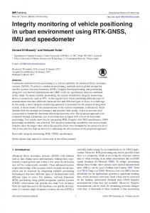
The solid line of Fig. 4 depicts the error of the primary position estimates for a 1400 meters measurement run using the processing steps described in section IV. The position error has both high frequency and low frequency behaviour.

High frequency errors not corresponding to the vehicle dynamics may be filtered out. This is done by combining the primary position estimates with knowledge about the expected speed and acceleration in a Kalman filter. The expected speed is a rough estimate, which we assume constant for a specific area. In a real system this estimate may be based on the speed limit, more specific knowledge of the traffic pattern or measured speed. The speed is thus input as a pseudo-measurement, yv , in the Kalman filter. The vehicle acceleration depends on the engine power and the driver’s usage of the accelerator pedal. We assume the acceleration to have low frequency behaviour and we model it as a 1. order Markov process. We expect coloured speed- and position-measurementerrors. A common approach is to model these as 1. order Markov processes in an augmented Kalman filter.

where y (l ) =  y p (l ) yv (l )  is the observations of position

A. System Description

in section IV.

T

and speed respectively. The observation matrix D is given by 1 0 0 1 0  D=  0 1 0 0 1 

and w (l ) =  w p (l ) wv (l )  is discrete white noise in the position- and speed-measurements respectively. B. The Kalman Filter The state space equation (5) and the process-noise covariance matrix is converted to discrete time as shown in chapter 5.3 of [12]. The Kalman filter is implemented as described in chapter 5.5 of [12]. This defines an algorithm capable of filtering the one-dimensional position estimates, y p , from the pattern recognition process described

The linear state space equation for a continuously dynamic system is defined as x& (t ) = Ax (t ) + Cv (t )

where

the

x (t ) =  x p (t )

state xv (t )

vector

(5) is

given

by

T

xa (t ) ∆p (t ) ∆v(t )  .

Its

components represent position, speed, acceleration, lowfrequency positionand speed-measurement-error respectively. The system matrix A and the process noise matrix C becomes 1 0

0 1 1 0 − Ta

0 0

0 0

0 0 0 1 − Tp 0

0  0  0 0  0 0 0    and C = 1 0   0  0 1  0 0  1 −  Tv 

Primary and KF Position Error 100 Primary estimates KF estimates

90 80

0 0  0  0 1 

70 60 50 40 30 20 10

where Ta represents the acceleration time-constant of the 1. order Markov process. Tp and Tv represent position- and speed-measurement-error time-constants for the 1. order Markov processes respectively. The process noise vector v (t ) =  va (t ) v p (t ) vv (t ) 

T

consists of corresponding continuous white noise for the three Markov processes. The observations at discrete time steps l are linear in the state variables such that y (l ) = Dx (l ) + w (l )

RESULTS

The system described above has been tested using about 30 km of CIR measurements from 4 routes in urban and suburban areas of Munich. The routes are between 450 to 850 meters of length. The same routes were driven several times. One of the measurement series from each route was processed to serve as the database. Comparison was then performed with the other measurement series from the same route.

Error [m]

0 0   0 A=  0   0 

VI.

(6)

0 0

50

100

150

200

250

Time [s]

Fig. 4. Primary and KF position error of a 1400 meters measurement run

A parametric search was performed for the exponent η used in the Box-Cox metric (3). The goal was to minimise the primary positioning error of the pattern recognition process. The best value was found to be η = 0.1. The nature of the results is such that a separation into three categories A, B and C is appropriate. For the series in category A the comparison process worked well and the secondary Kalman filtering further enhanced the accuracy. For the series in category B the comparison process

performed worse and the error was more difficult to model. In category C comparison was not possible using the algorithm described above. Table I yields an overview of the number of series in each category and the corresponding sum of measured kilometres.

Category # series Total km

TABLE I OVERVIEW OF POSITION ACCURACY A B 18 16 9.7 km 8.8 km

C 20 10.3 km

AKNOWLEDGMENT

# signify “number of”

1

1 0.9 Comulative distribution

Comulative distribution

Fig. 5 depicts the position-error cumulative distribution function (CDF) for the 18 series in category A and the 16 series in category B. The accuracy for the category A series is such that 67 percent of the position estimates are within 17.5 meters of the true positions and 95 percent of the position estimates are within 50.1 meters of the true positions. For the category B series 67 percent of the position estimates are within 46.3 meters of the true positions and 95 percent of the position estimates are within 87.6 meters of the true positions.

0.9 0.8 0.7 0.6 0.5 Primary estimates: 67 perc: 27.4 m 95 perc: 82.6 m

0.4 0.3

Kalman estimates: 67 perc: 17.5 m 95 perc: 50.1 m

0.2 0.1 0 0

50

100

150

0.8 0.7 0.6 0.5 Primary estimates: 67 perc: 54.2 m 95 perc: 103 m

0.4 0.3

Kalman estimates: 67 perc: 46.3 m 95 perc: 87.6 m

0.2 0.1 200

0 0

Error [m]

50

100

150

200

Error [m]

Fig. 5. Position-error CDF of the 18 series of category A accuracy (left) and the 16 series of category B accuracy (right) VII.

location but separated in time. This seems to be harder to achieve for all times. The results show that very good (category A) and fairly good (category B) accuracy is obtained 64 percent of the time with signals from one BS only. More complex processing or other sources of location sensitive measurement data is required in order to further enhance the availability of this positioning method.

CONCLUSIONS

Channel impulse response (CIR) measurements were performed several times along routes in urban and suburban areas of Munich. The measurements were processed to yield a database of feature vectors. The vectors in the database were compared with feature vectors from other measurement runs. The primary position estimates from the comparison process were combined with knowledge about the vehicle dynamics in a Kalman filter, in an attempt to improve the overall accuracy. The accuracy of this method is primarily a function of two factors. The first is the problem with similar nearby CIR measurements. This seems to be handled well by the secondary estimation procedure, the Kalman filter. The second is the problem with the reproducibility of the CIR. By this we mean the ability to measure two relatively similar CIRs, according to our pattern recognition, at the same

We would like to thank Siemens AG in Münich for providing the channel measurements used in this research. REFERENCES [1] "Third Report and Order," United States Federal Communications Commission CC Docket No. 94-102, Oct. 1999. [2] G. M. Djuknic and R. Richton, "Geolocation and assisted GPS," Computer, vol. 34, pp. 123-125, Feb 2001. [3] M. Lindsey, G. Bilgic, G. Davis, B. Fox, R. Jensen, T. Lunn, M. McDonald, and W. C. Peng, "GSM Mobile Location Systems," Omnipoint Tech. Inc. July 1999. [4] D. Porcino, "Location of Third Generation Mobile Devices: A comparison between Terrestrial and Satellite Positioning Systems," presented at VTC 2001 Spring, Rhodes, Greece, May 2001. [5] H. Koshima and J. Hoshen, "Personal Locator Service Emerge," IEEE Spectrum, Feb. 2000. [6] P. Dana, "Global Positioning System Overview," Dep. of Geography, The University of Colorado at Boulder 1994. [7] H. Laitinen, J. Lähteenmäki, and T. Nordström, "Database Correlation Method for GSM Location," presented at VTC 2001 Spring, Rhodes, Greece, May 2001. [8] J. G. Proakis, Digital Communications, 3 ed: McGrawHill, 1995. [9] T. Fehlhauer, P. W. Baier, W. Konig, and W. Mohr, "Optimized wideband system for unbiased mobile radio channel sounding with periodic spread spectrum signals," presented at IEICE Trans. on Communications, Japan, 1993. [10] T. Nypan, K. Gade, and T. Maseng, "Location using Estimated Impulse Responses in a Mobile Communication System," presented at NORSIG, Trondheim, Norway, Oct 2001. [11] R. Van der Heiden and F. C. A. Groen, "The Box-Cox Metric for Nearest Neighbour Classification Improvement," Pattern Recognition, vol. 30, pp. 273279, 1997. [12] R. G. Brown and P. Y. C. Hwang, Introduction to Random Signals and Applied Kalman Filtering, 3 ed: John Wiley & Sons, 1997.